Part 1: Fit a Neural Field to a 2D Image
In this section, I implement Neural Radiance Field in 2 dimensions. In 2 dimensions, we don't have the concept of radiance so essentially Neural Radiance Field in 2 dimensions reduces to Neural Field, in which we represent 2D by mapping (u,v) to (R,G,B) - converting the pixel coordinate to RGB values. For this, I created Multilayer Perceptron and Sinusoidal Positional Encoding with given architecture. For Multilayer Perceptron, I used 4 hidden layers(size 256) with RELU and a linear layer(size 3) with sigmoid. Also, I created a dataloader that randomly samples certain number of pixels from the image at each iteration. To determine the correct hyperparameters, I have explored different values for learning rate and max frequency L for the given image. As the baseline, I used the hyperparameters layers=4, hidden dim=256, L=10, LR=1e-2. Firstly, I explored the effect of max frequency L. Here are my results for the baseline, L=20, LR=5:
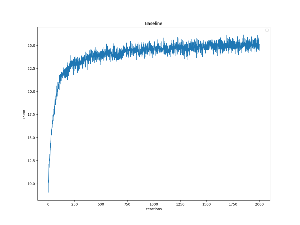
Baseline PSNR Curve
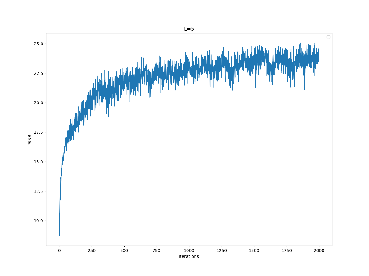
L=5 PSNR Curve
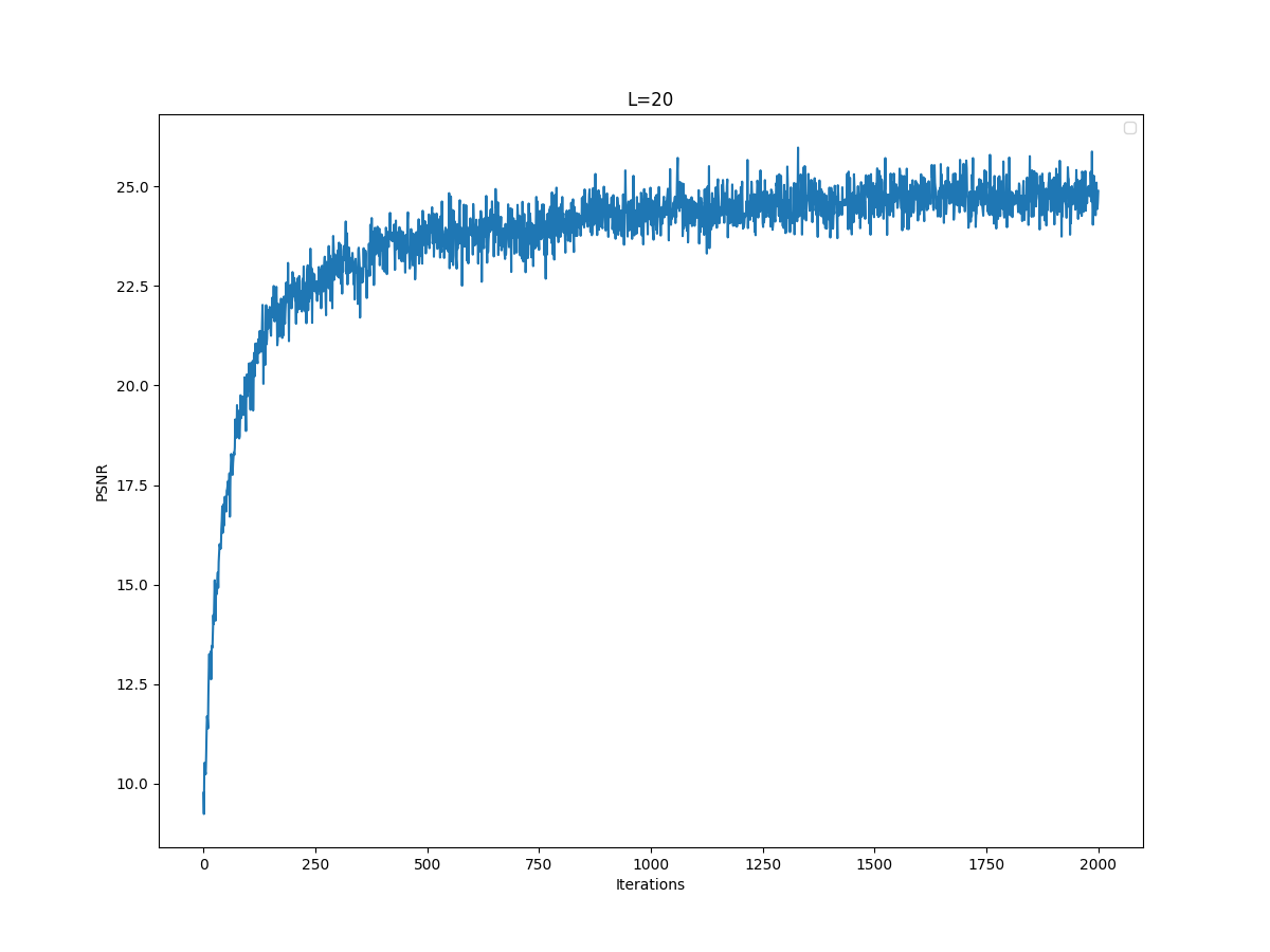
L=20 PSNR Curve
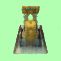
Baseline Final Image

L=5 Final Image

L=20 Final Image
From the images, it is clear that reducing the max frequency from 10 to 5 resulted in worse performance. Also, the increase from 10 to 20 did not improve the model's performance visibly, PSNR curves seemed to converge to similar value. Thus, I decided to use L=10.
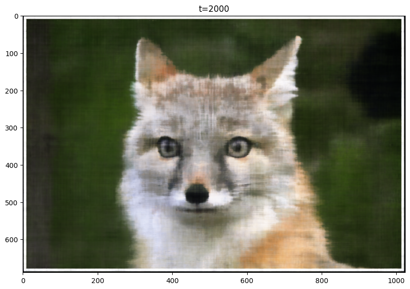
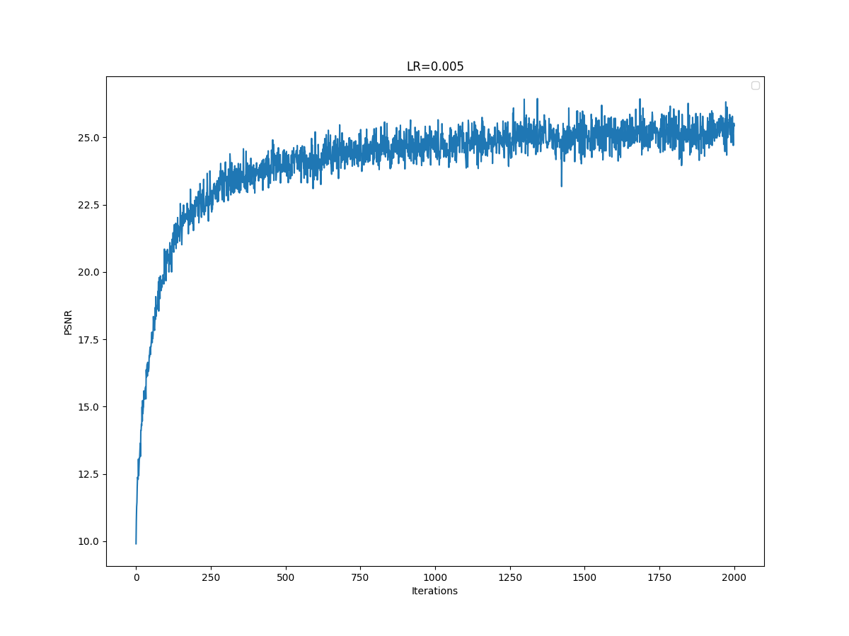
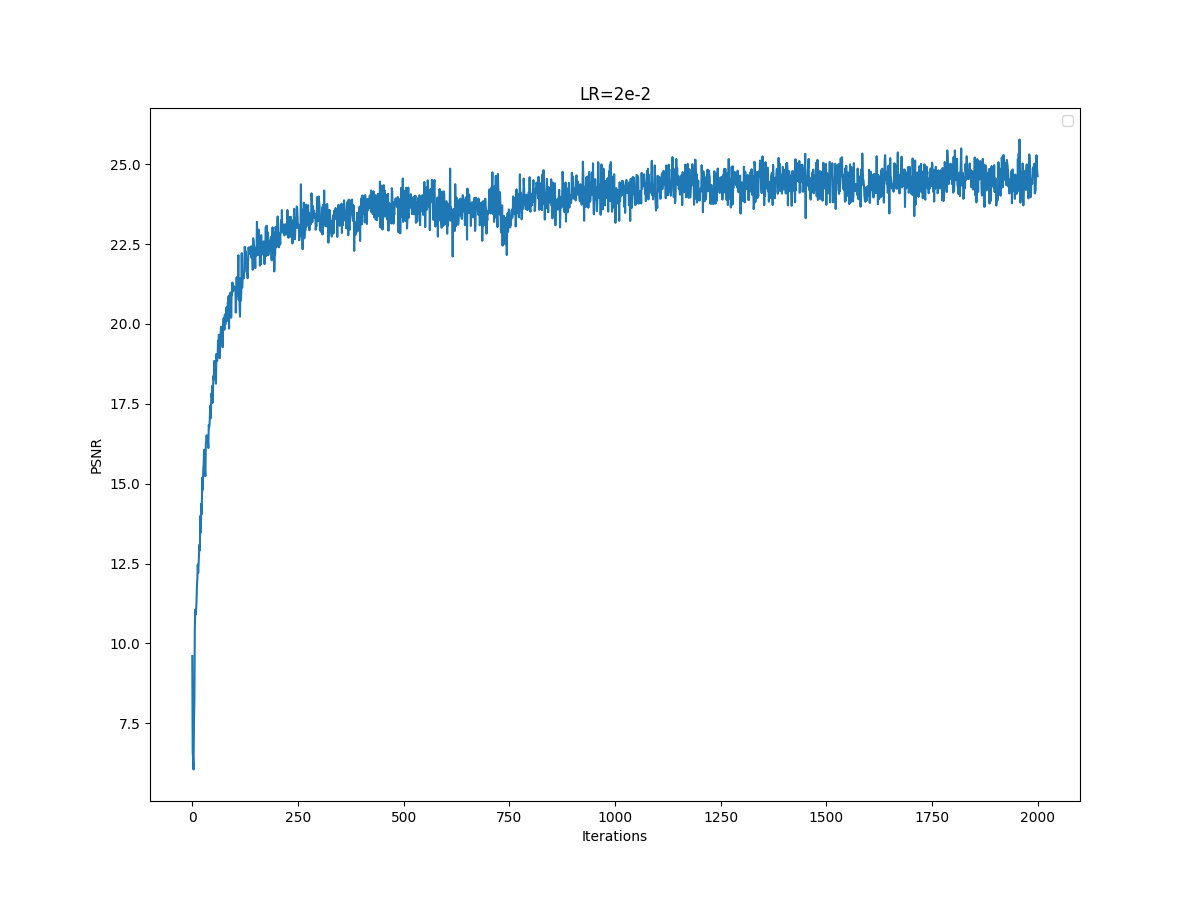
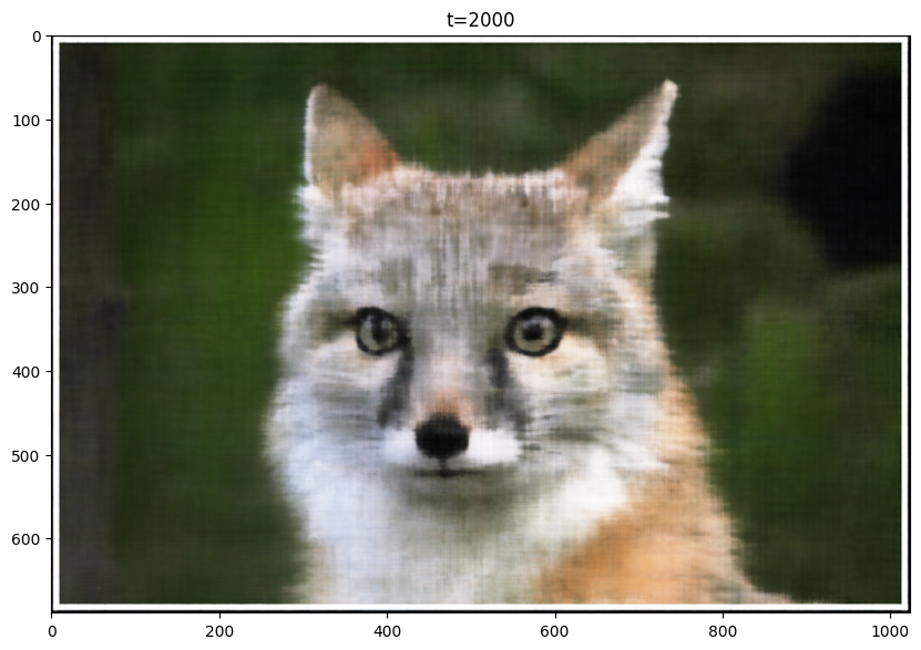
As another hyperparameter, I varying the learning rate. Here are my results for the baseline, LR=0.02, L=0.005:
Baseline PSNR Curve
LR= 0.005 PSNR Curve
LR=0.02 PSNR Curve
Baseline Final Image
LR=0.005 Final Image
LR = 0.02 Final Image
Training curves look pretty similar, but halving the learning rate caused a slight drop in performance. Also, for learning rate 2e-2, I think the final image has worse quality than the final image for the baseline.
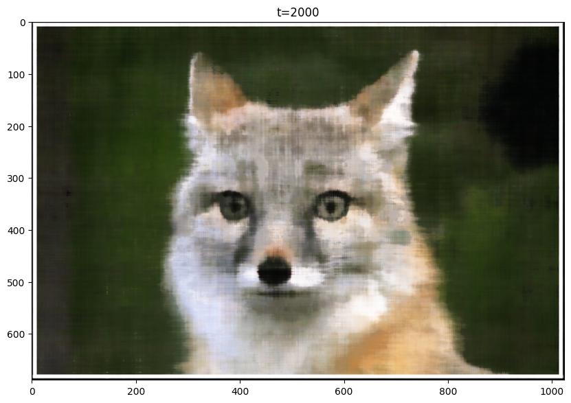
Here are my results for the given image, sampled at every 400 iterations. I trained the model for 2001 iterations. For this training, I used the following hyperparameters, layers=4, hidden dim=256, L=10, LR=1e-2:
Training PSNR Curve
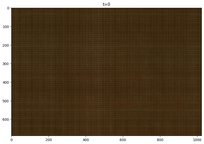
T=0
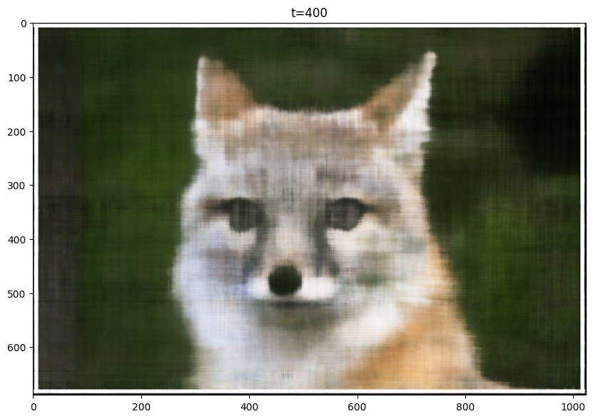
T=400

T=800

T=1200
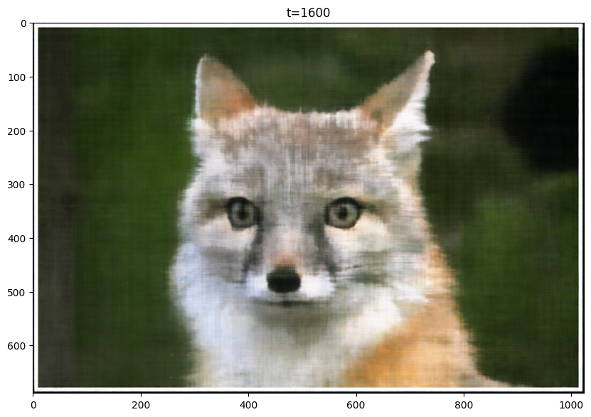
T=1600

T=2000
I also ran my training loop for another image of my choosing, a crocodile. For this training, I used the following hyperparameters, layers=4, hidden dim=256, L=10, LR=5e-3:. Here are my results for the image, and my training curve:
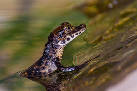
Original Image
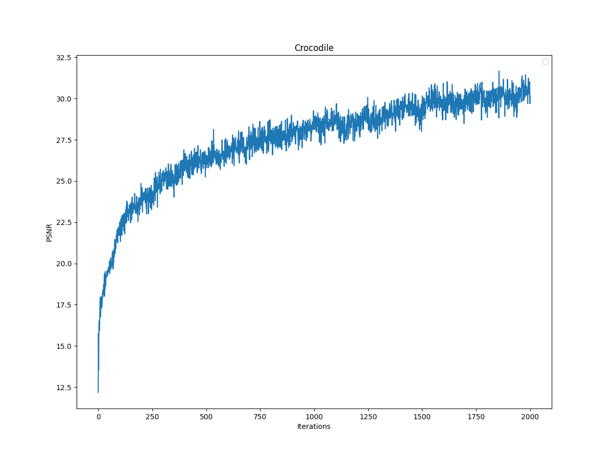
Training PSNR Curve
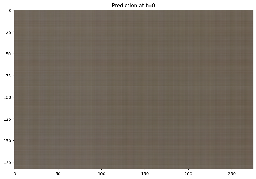
T=0
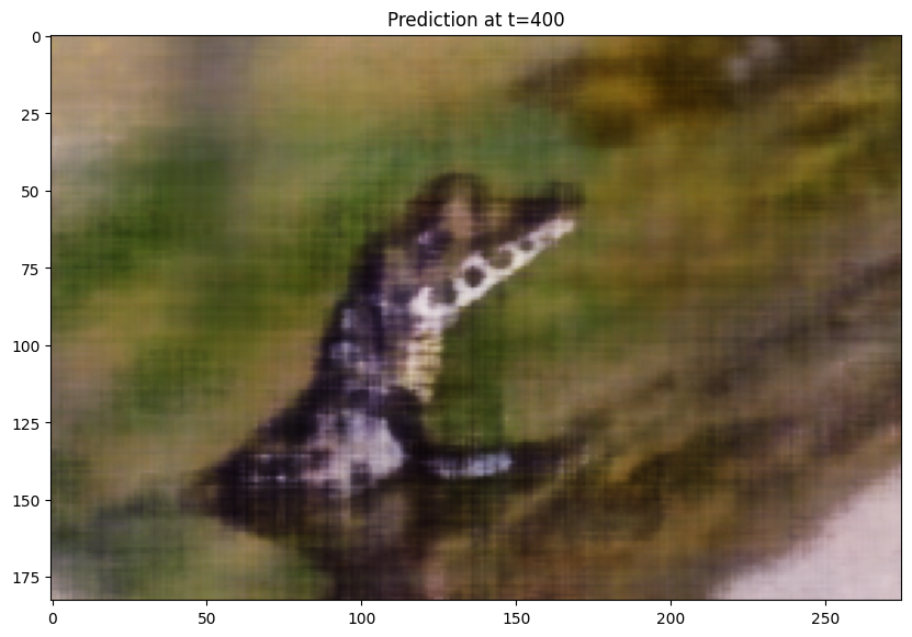
T=400
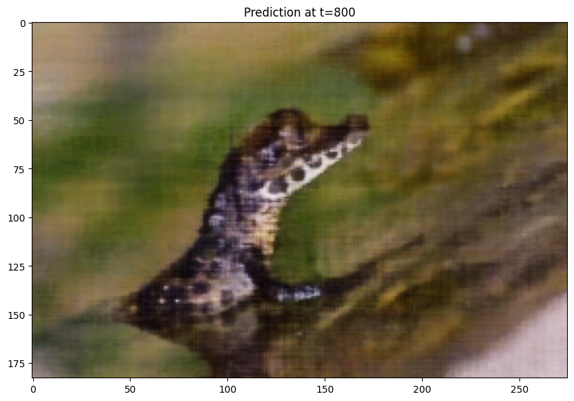
T=800
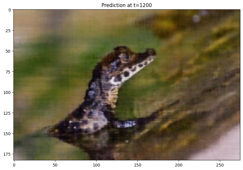
T=1200
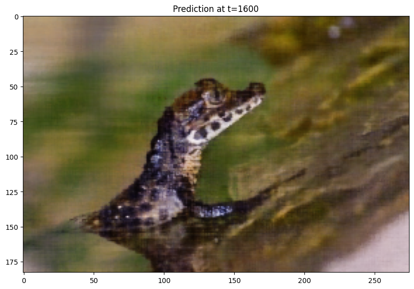
T=1600
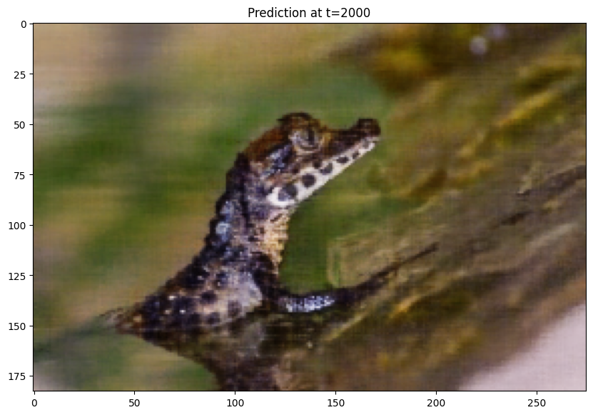
T=2000
Part 2: Fit a Neural Radiance Field from Multi-view Images
In this part, I will use a neural radiance field to represent 3D. For this, I will use inverse rendering for multi-view calibrated images.
Part 2.1: Create Rays from Cameras
In this part, I create two functions for sampling, sample_rays(self, numberofrays, numberofimages) and sample_along_rays(rays_o, rays_d, perturb). I defined the sample_rays function under RaysData class. Similar to Part 1, sample_rays randomly samples numberofrays from numberofimages. sample_along_rays is used for sampling points along the obtained rays, and optionally perturbed in training so that every location along the ray would be covered.
Part 2.2: Sampling
In this part, I defined the required functions, transform(c2w, x_c), pixel_to_camera(c2w, x_c), pixel_to_ray(K, c2w, x_c). transform function takes in camera coordinates and obtains the corresponding world coordinates using c2w matrix. pixel_to_camera takes in pixel coordinates and obtains camera coordinates, using the intrinsic matrix K. pixel_to_ray takes in world coordinates, and by using the other functions, obtains rays with origin and normalized directions.
Part 2.3: Putting the Dataloading All Together
In this part, I put everything I did so far together to visualize the given tests:
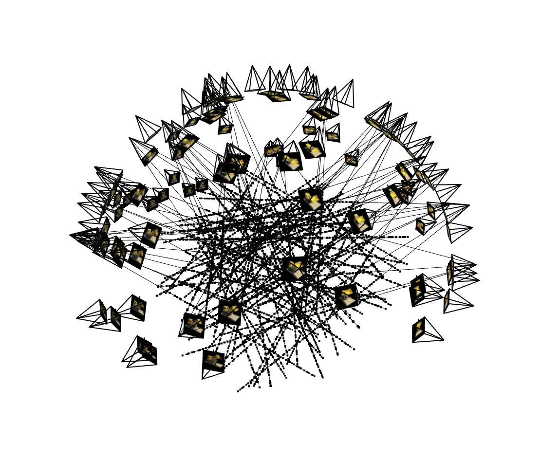
Cameras, 100 Rays, Samples
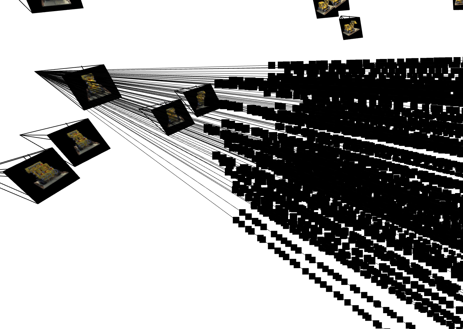
Random rays from the first image
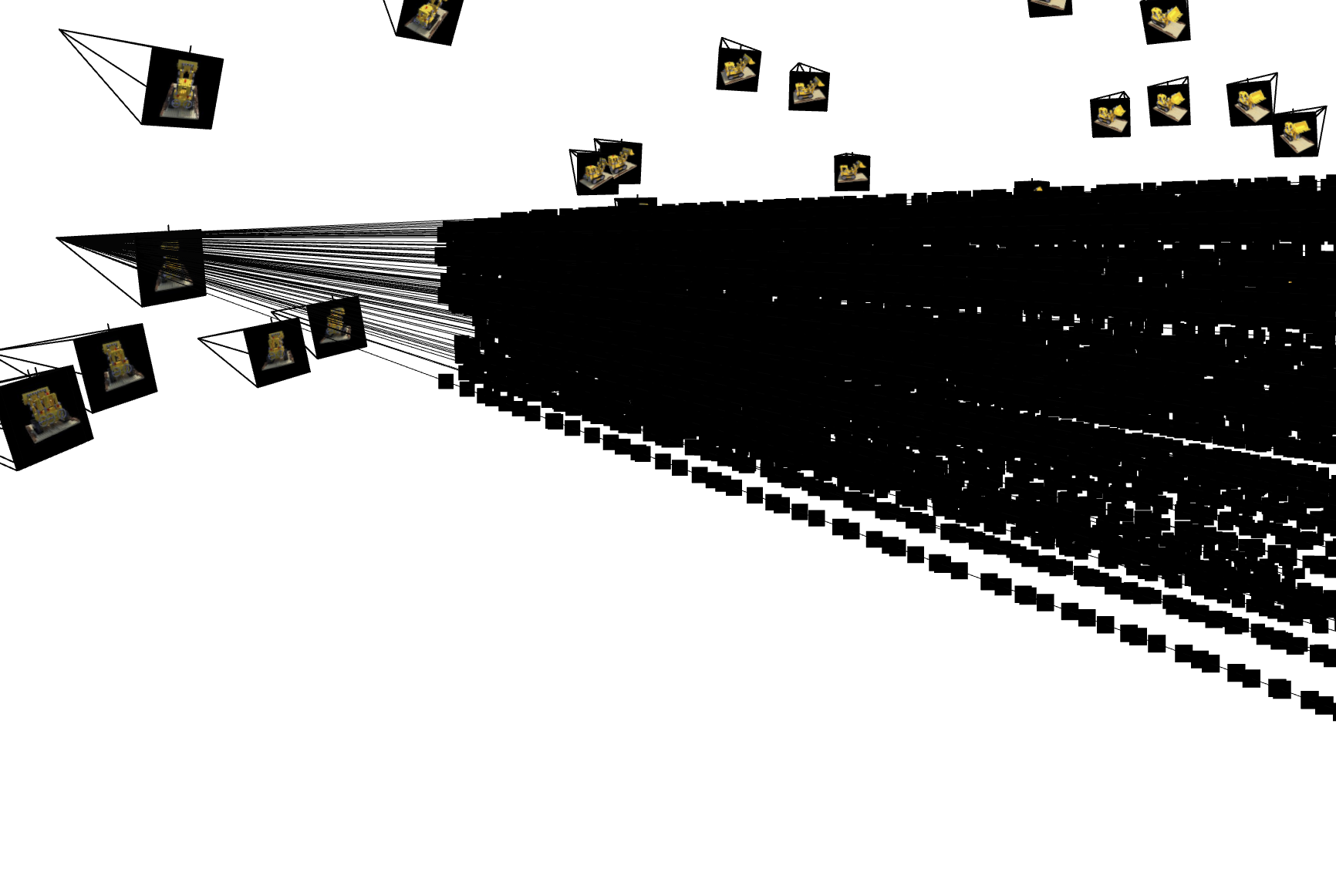
Random rays from the top left corner of the image
Part 2.4: Neural Radiance Field
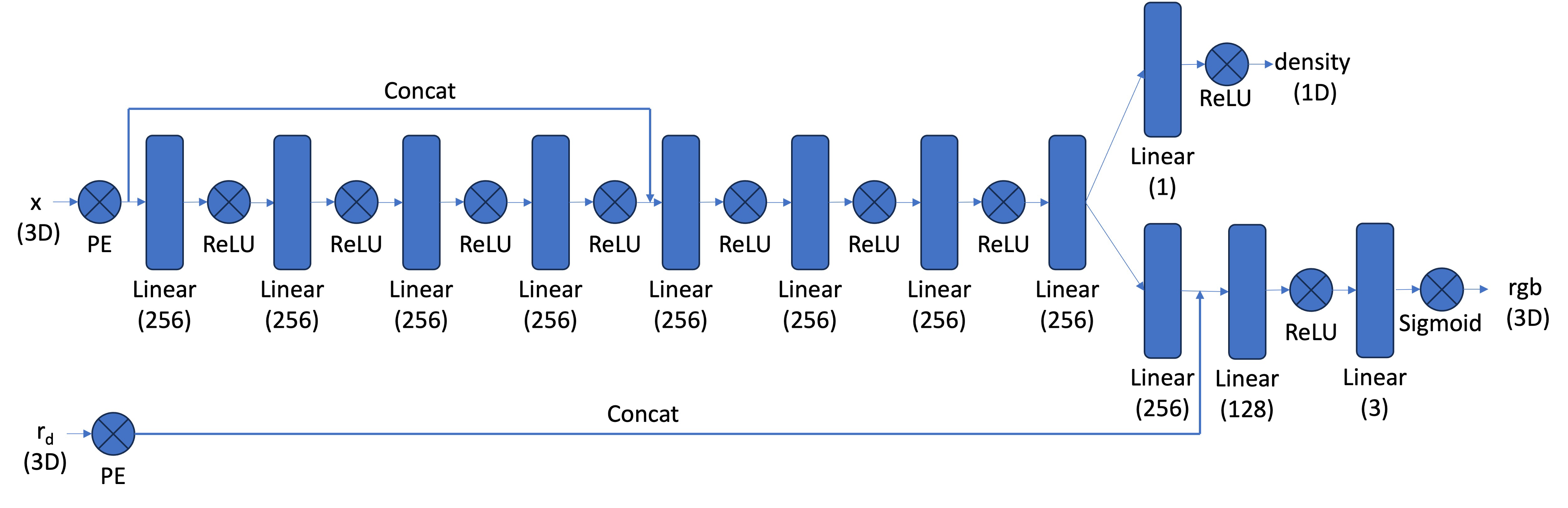
In this part, I implement the NeRF architecture. It is similar to MLP but there are some changes as we have samples in 3D, and want to predict density and color of the samples. One of the main changes are now the MLP is deeper because the task we are trying to implement is harder. Also, we are not only going to output color but also density for the inputs, which are 3D world coordinates and ray direction. For this, I will use the direction as the condition to output colors. Lastly, I inject the input to the middle of the MLP after getting it through PE I defined earlier to make model not forget about the input as the neural network got deeper. For this part, I used the given architecture:
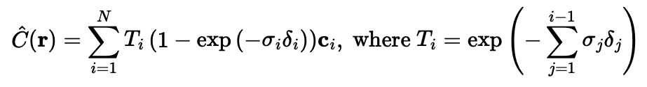
Part 2.5: Volume Rendering
In order to obtain render colors, I used the given volume rendering equation, which combined the batches of samples from each ray:
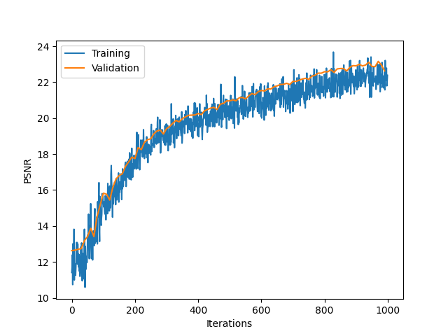
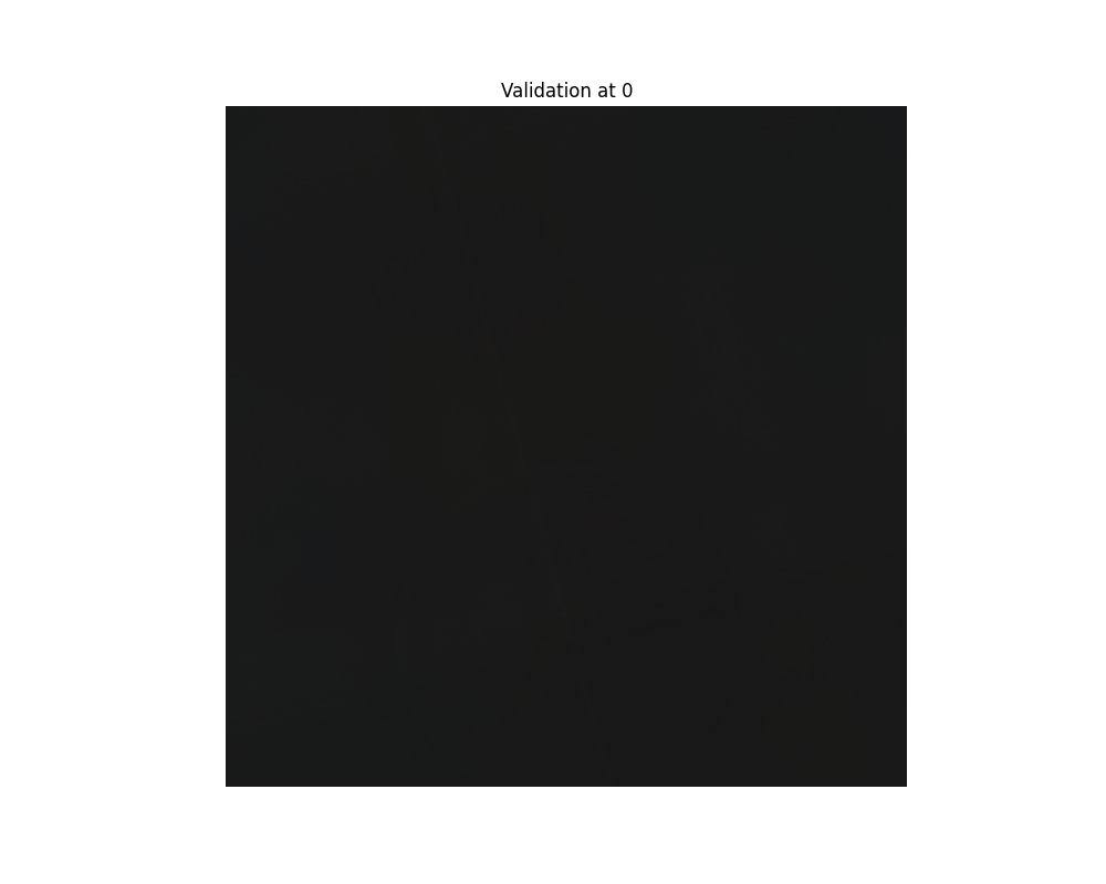
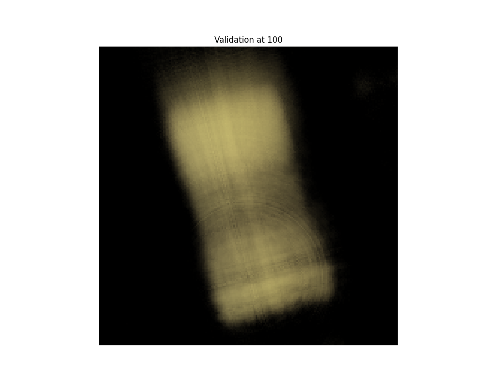
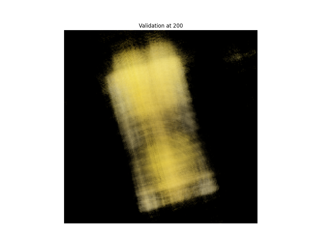
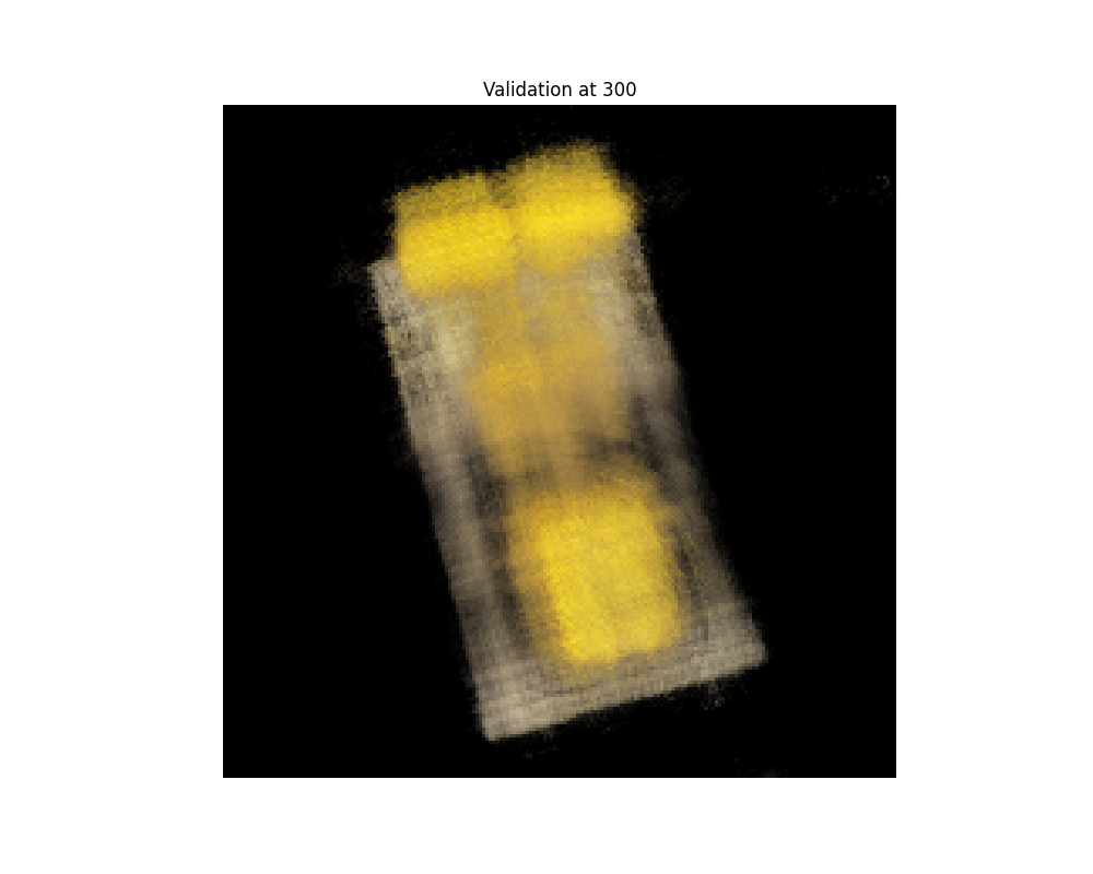
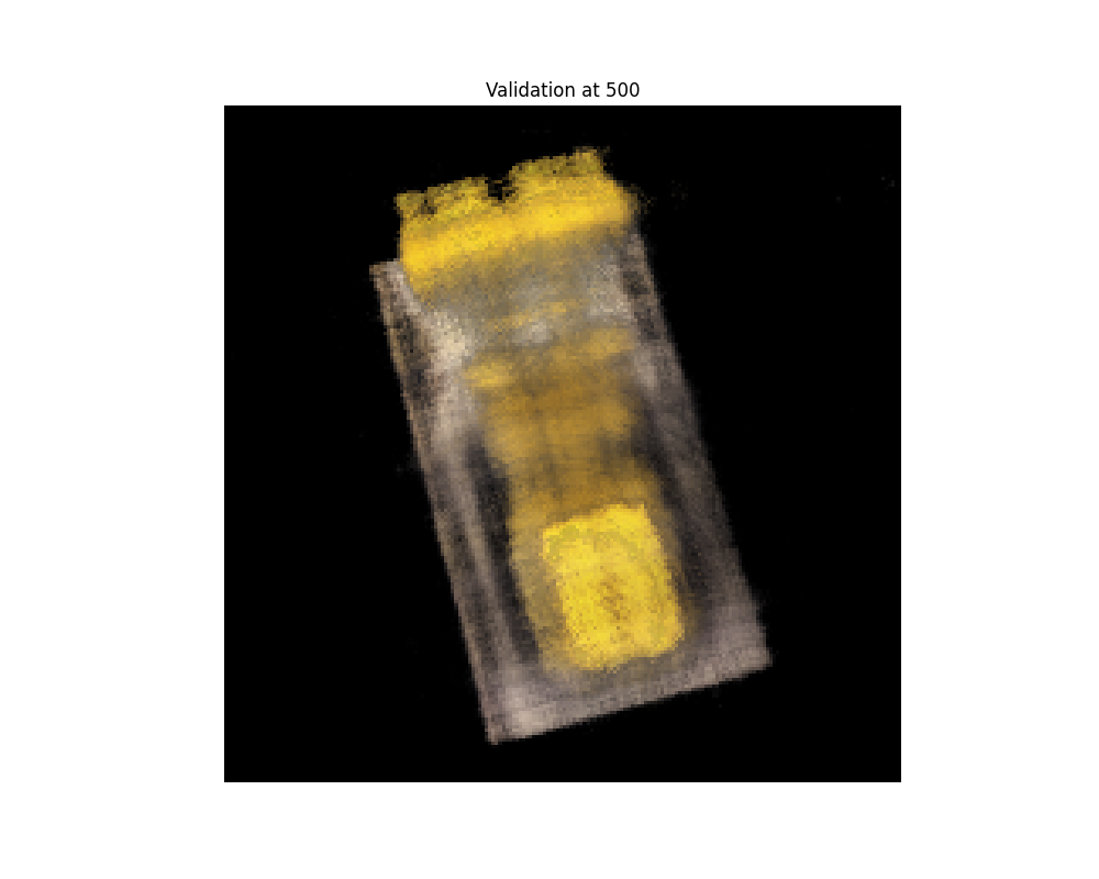
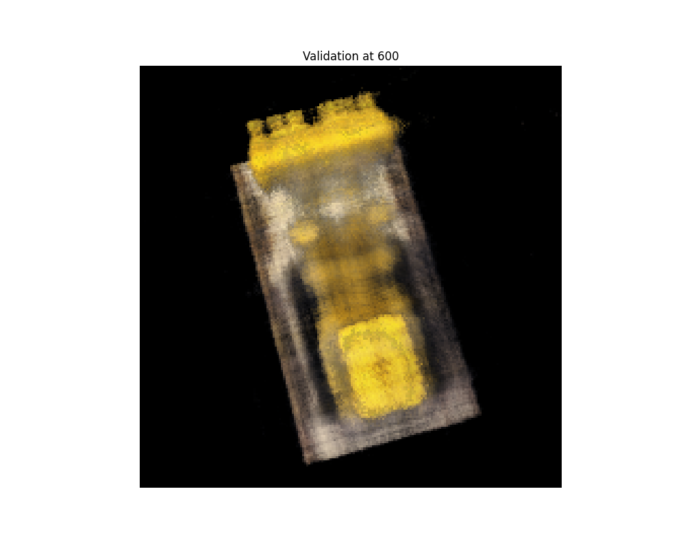
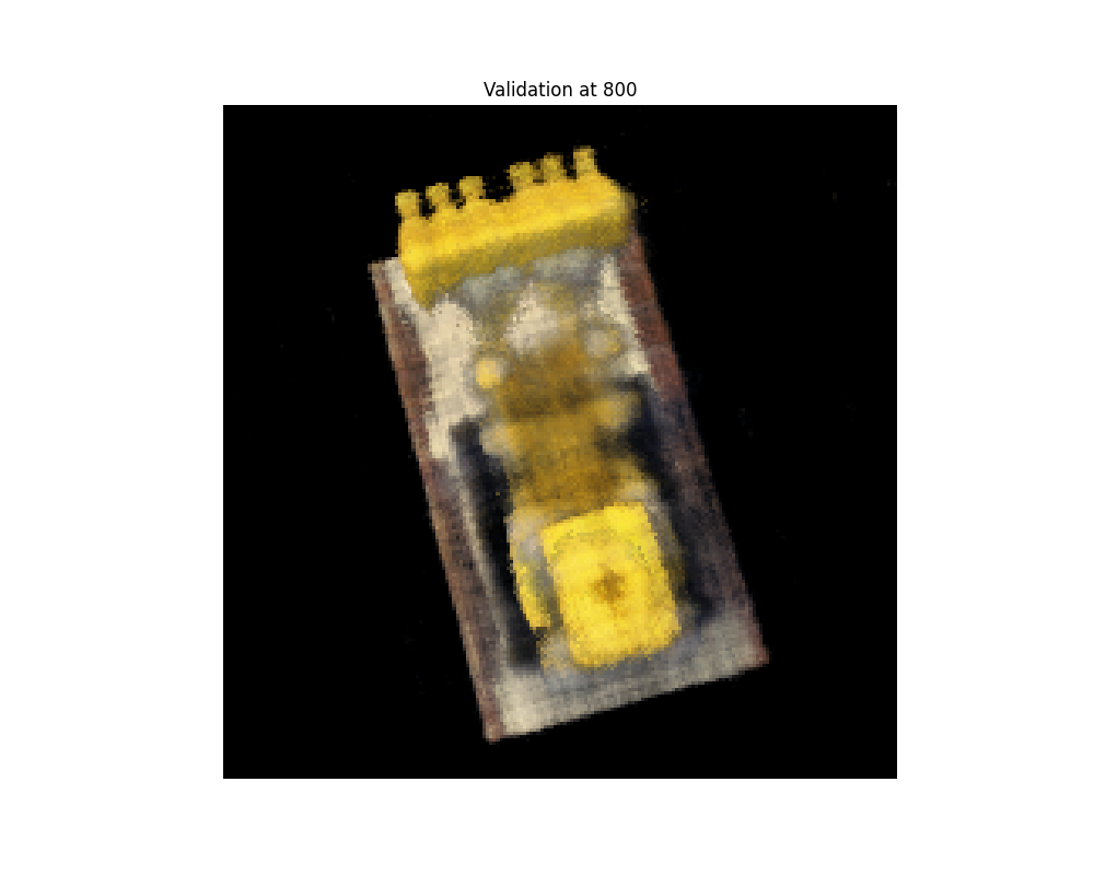
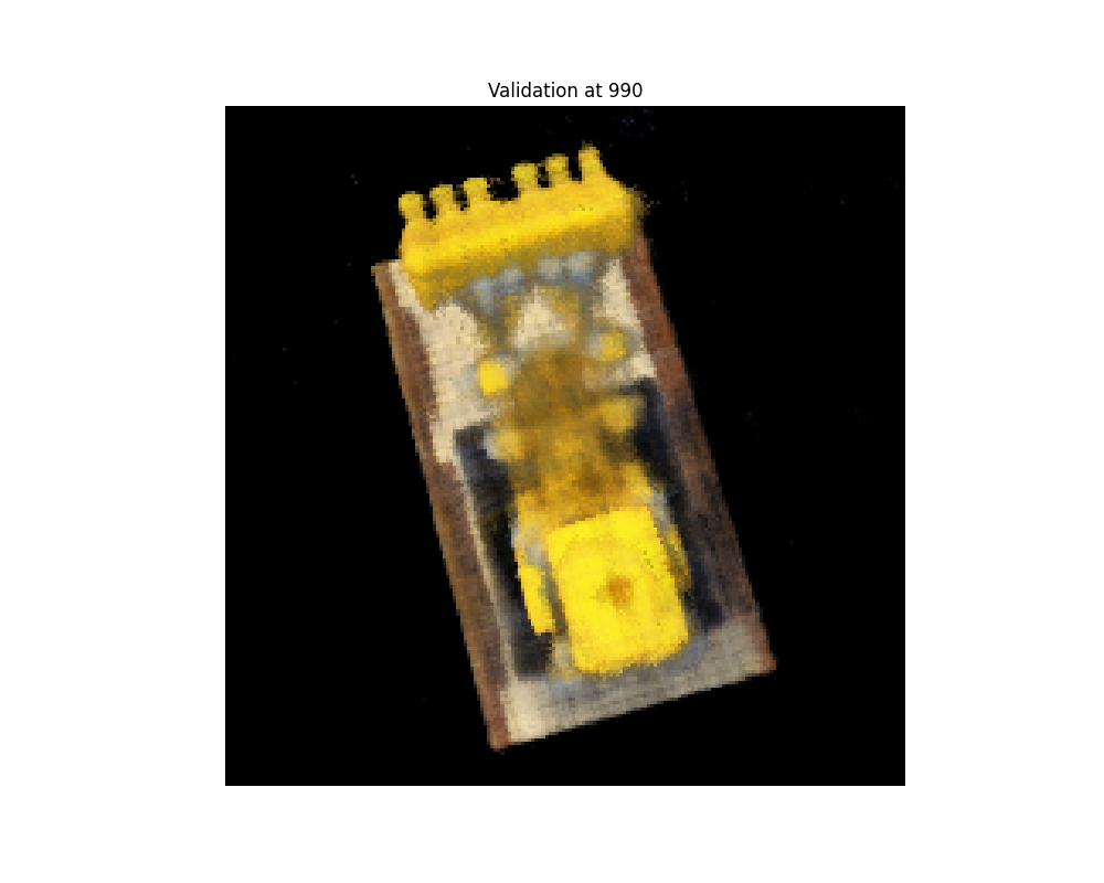
Here is the visualized training, predictions shown for each 100 iterations. I used the given hyperparameters, and trained the model for 1000 iterations. Also, I provide the PSNR curve on the validation set (every 10 iterations) and the training set.


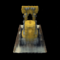
Combining everything together, here is a spherical rendering of lego using the provided camera extrinsics:
B&W: Background Coloring
For bells and whistles, I implement the background color. The background color is added to the rendered scene by treating it as the color seen when a ray passes through all objects without being blocked: