Shoot the Pictures

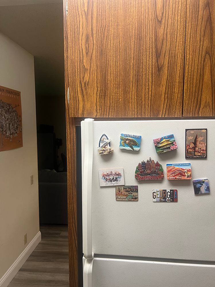
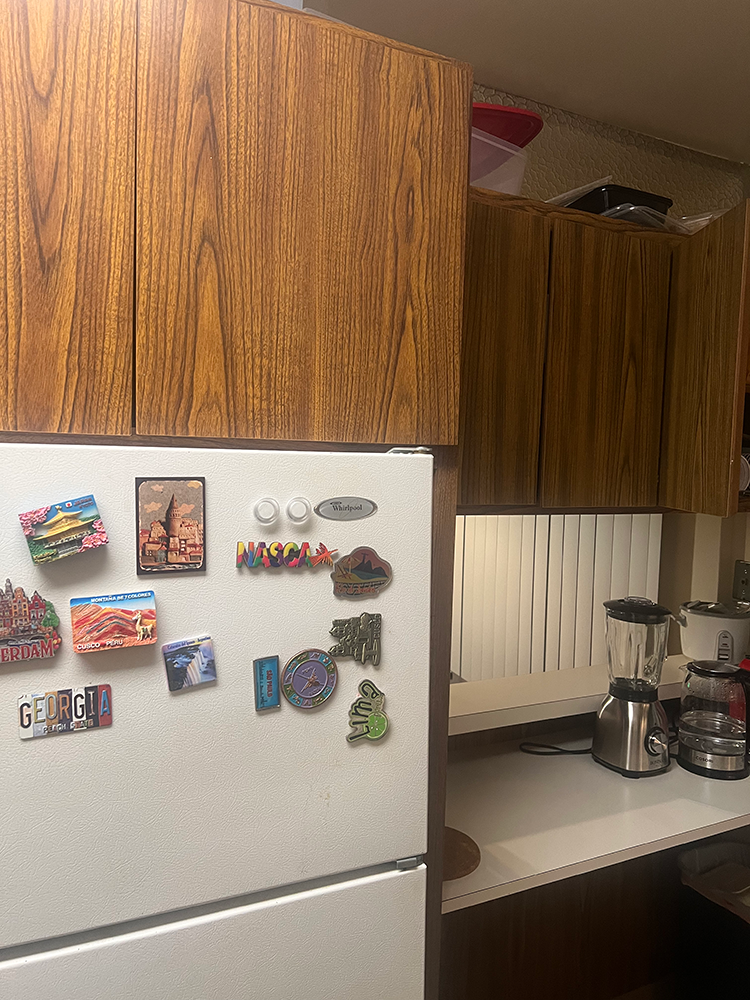
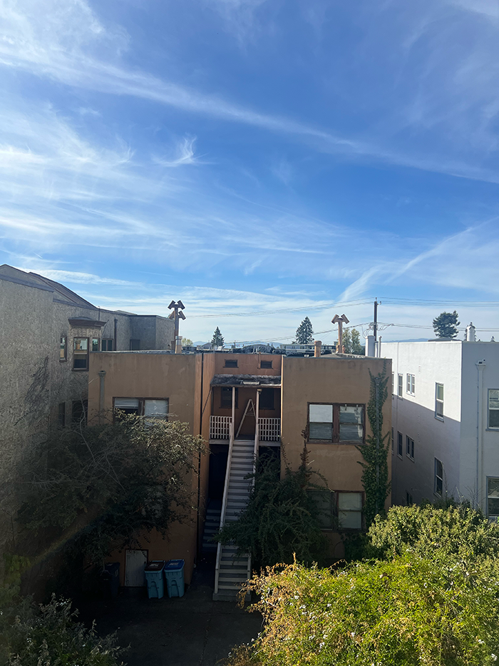
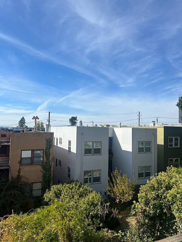
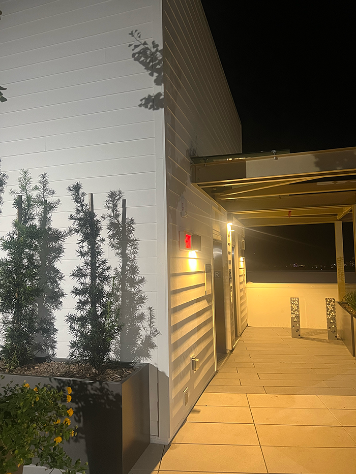
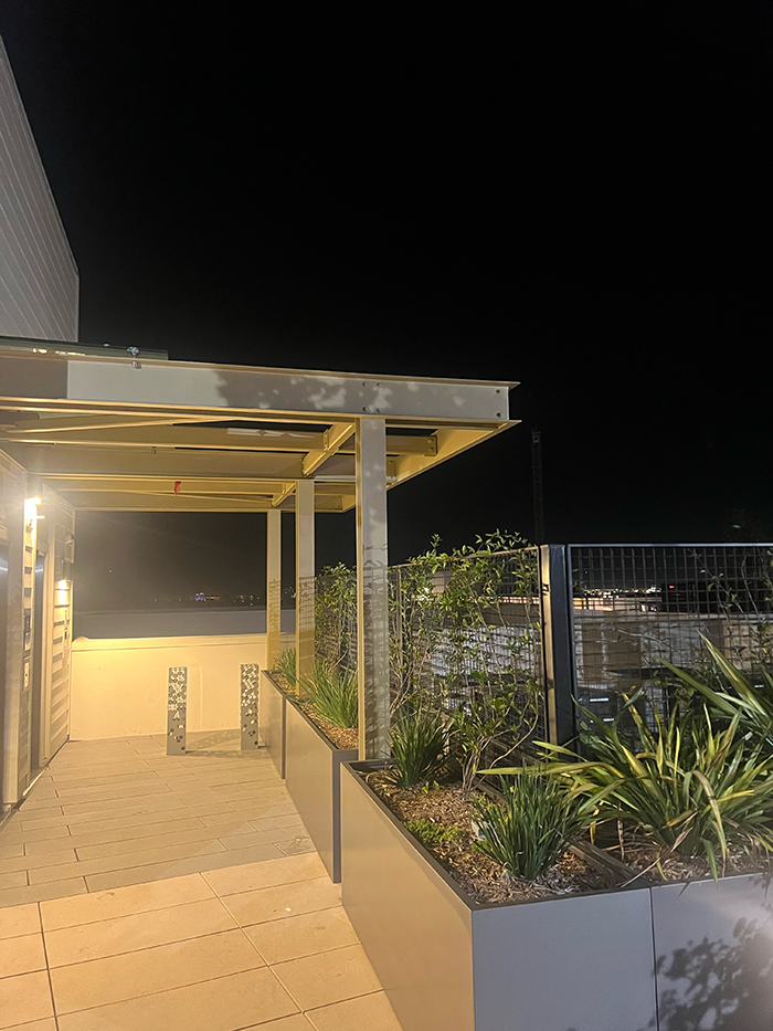
Here are the pictures I used for this project:

Recover Homographies

To recover homographies, we want to find the projective transformation that transforms coordinates of a point with an augmented coordinate (x, y, 1) to another augmented coordinates with the same center of projection (x', y', w). When we set the scaling factor to 1, we have the following equation:

If we expand out the equations and divide wx' and wy' by w:

If we multiply both sides by the denominator and keep x' and y' at one side, we would get equations for x' and y' in terms of other variables, including themselves. We can write the same equations for different corresponding points, if we stack them together:

However, ideally, we should use more than 4 correspondence points to make homography recovery stable and less prone to error. Using more than 4 correspondence points would make the equation overdetermined and we solve this by least-squares solver to recover the homographies. For this project, I used the given correspondence tool to select the correspondence points.

Warp the Images/Image Rectification

After calculating the homography, I use inverse warping to warp original images to the desired shape. Since I use inverse warping, the corresponding pixels in the source image can be lie between pixels so I used RegularGridInterpolator to interpolate the pixel values.

For image rectification I used the inverse warping with homography I calculated earlier. Instead of selecting corresponding points between two images, I chose the edges of a rectangle or a square shape from an image and I manually defined the corresponding points so that these edges would form a rectified rectangular shape. Here are the corresponding points I have chosen and the resultant rectified images:

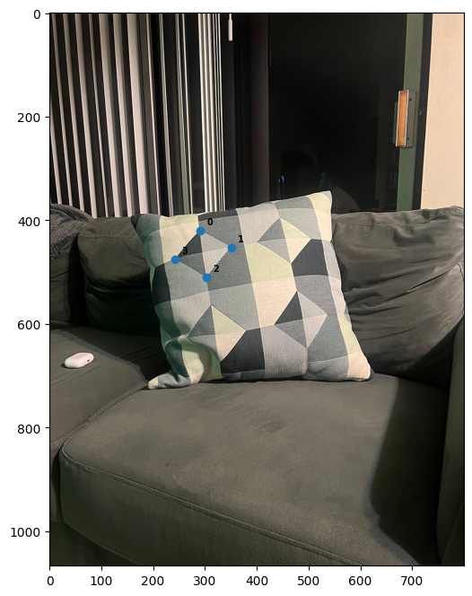
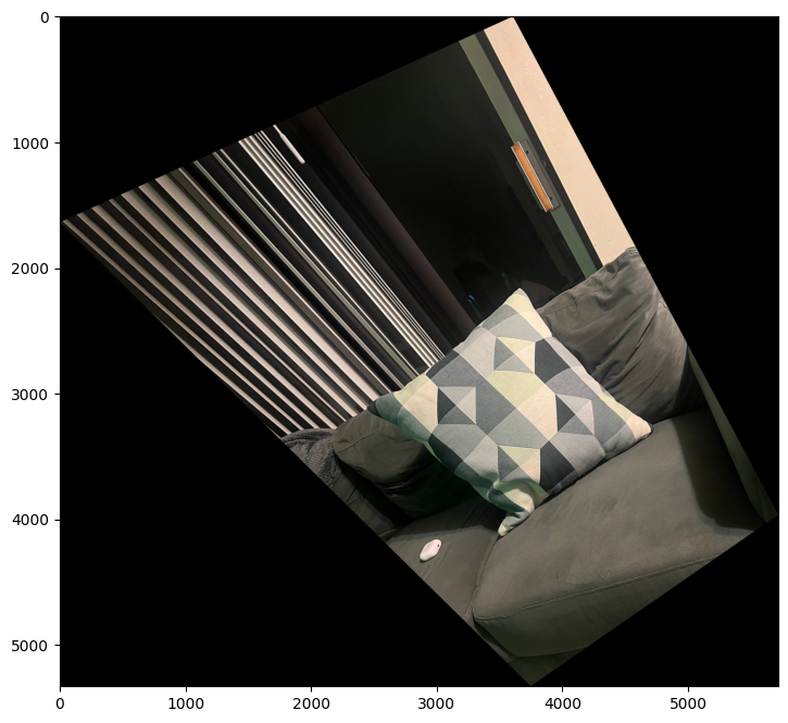
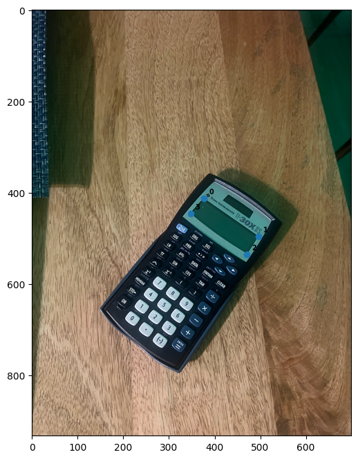
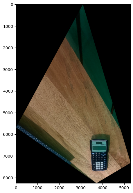
For the first image, I have manually chosen the corresponding points to be [[200,200],[500,200],[500,500],[200,500]] to form a square. For the second iamge, I have manually chosen the corresponding points to be [[200,200],[800,200],[800,400],[200,400]] to form a rectangle.

Blend the images into a mosaic

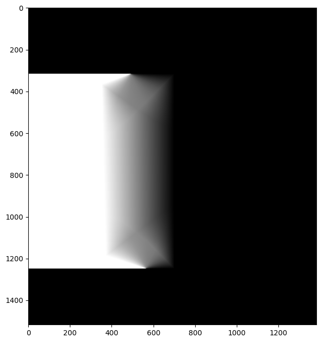
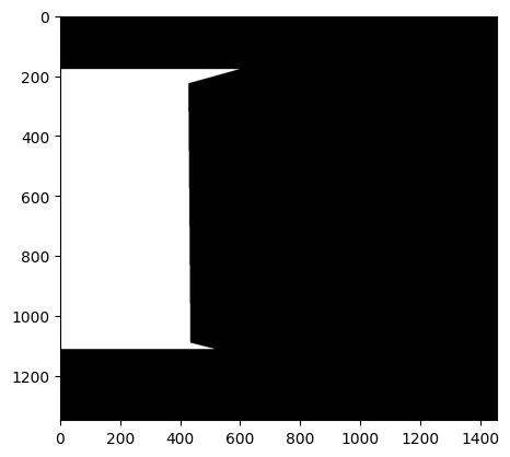
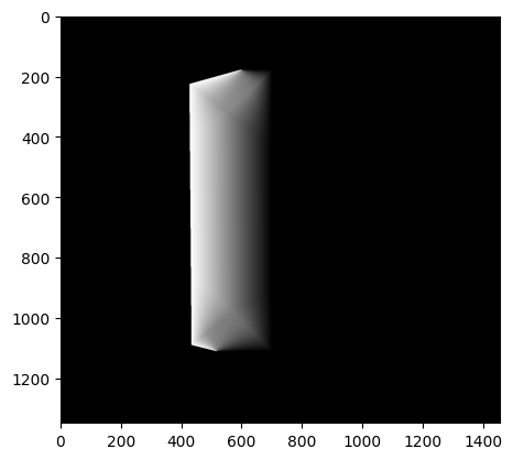
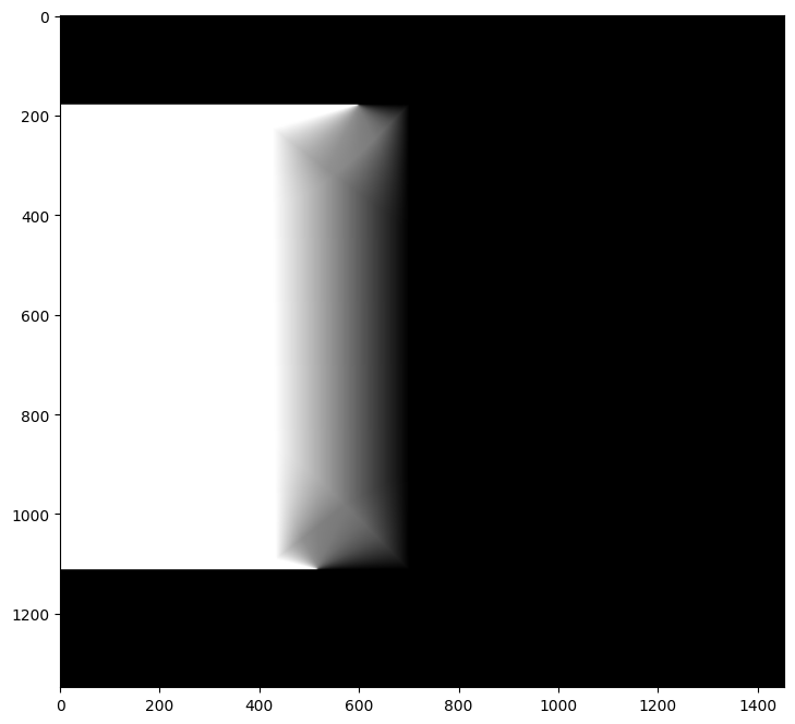
To blend the images into a mosaic, firstly, I warped one of the images based on the correspondence points. Before warping, I calculate the final image's shape and align the warped image with the original image by calculating if there is any offsets. Then, I created indicator masks for both the original and warped image in the final image's shape. These masks set pixels to 1 if there is a corresponding pixel in the original or warped image. I found the overlapping pixels between the two images using these masks. After finding the overlapping pixels, I used a Laplacian stack for blending. For a Laplacian stack, we need a mask for the images to blend. I separated the mask into two parts. The first part is the non-overlapping pixels for the original image. Since there is no overlap between the images at these pixels, I used the indicator mask I created for the images at these pixels. For the overlapping pixels, the computation is more complicated. I used cv2.distanceTransform to calculate distance to non-overlapping pixels from both images for each overlapping pixel. Then, I found the ratio of distance2/(distance2+distance1) for each overlapping pixel where distance1 indicates the distance to the closest non-overlapping pixel in the original image. By combining these two parts, I create the mask for the Laplacian stack:

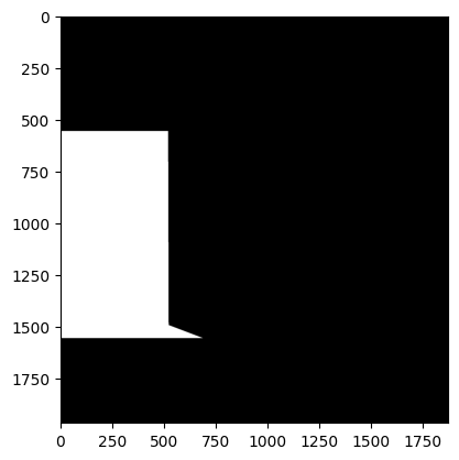
Non-overlap part of the mask

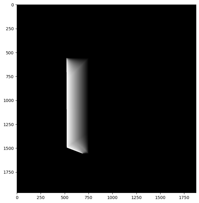
Overlap part of the mask

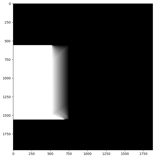
Full mask

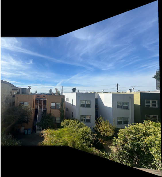
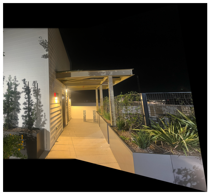
After creating the mask, I used a Laplacian stack with original and warped images padded to the final image's shape to create the mosaic:

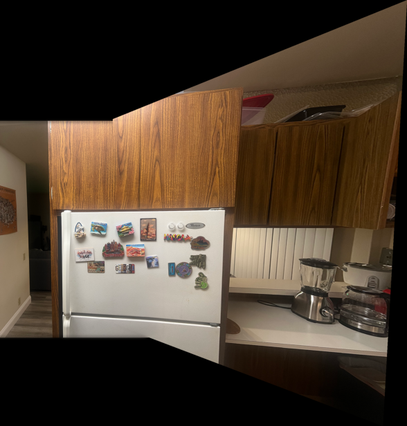
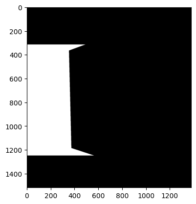
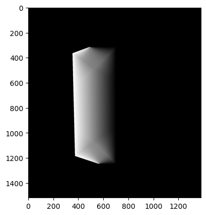
Here are other examples of mosaicing with their original images, mask, and the final blended image:

Part B

Detecting Corner Features

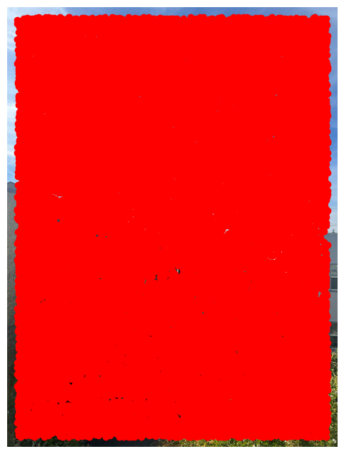
To detect the corner features, I used the given Harris Point detector. For one of my images, here is the points that Harris Point detector classified as likely to be corner features:

Adaptive Non-Maximal Suppression

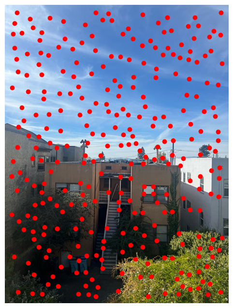
Even though Harris Point detector detects corner-like features, clearly, there are too much points and they are abundant. Thus, I use Adaptive Non-Maximal Suppression to extract features. To get correspondence points that are far away from each other and have strong corner features, we sort the distance based on the strength of their corner response. For each point, we calculate the distance to the closest point who has a stronger corner response. Then, we sort the points based on these distances and limit the number of features to be extracted to 300. Here is the result:

Extracting Feature Descriptors

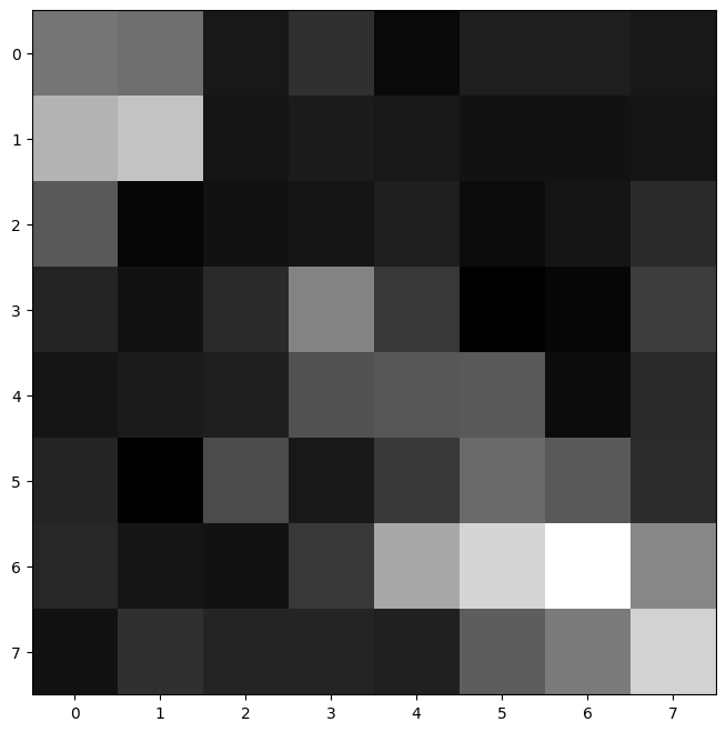
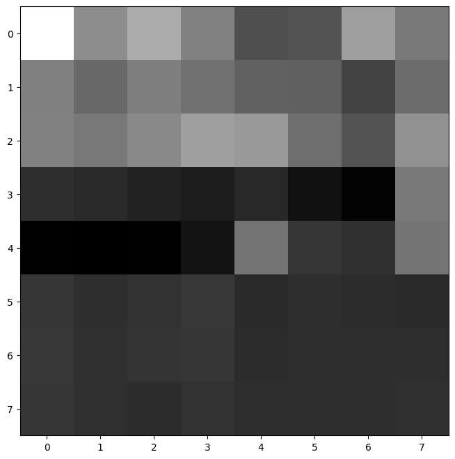
After identifying the features, now we have to extract feature descriptors. For each feature, we extract 40x40 windows, and downsample to get 8x8 patches. Before this step, low-pass Gaussian filter is applied. After getting the patches, each patch is normalized and reshaped to form 64 element feature descriptors for each feature. Here are some examples:

Matching Feature Descriptors

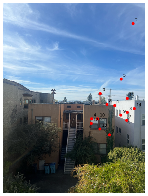
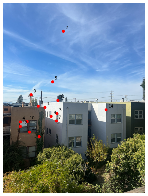
After extracting the feature descriptors for each image, we need to match them. I created k-d trees for each image. I query the closest 2 pairwise feature vectors for each feature in one of the images. I calculated the L2 norm distance ratio of these 2 vectors to the original features. Using Lowe's trick, I only keep the closest feature vectors that have less a certain threshold distance ratio and also checked with the other tree to ensure that original feature vector is also the closest feature vector for the chosen feature. This greatly reduced the outliers, and here is the filtered matches:

Robust method (RANSAC) to Compute Homography

To further reduce the outliers and inconsistencies, I implement the RANSAC algorithm. For 1000 iterations, I choose 4 matched point pairs and calculate homography based on them. Then, I calculated the inliners -- points that their transformed points are with a certain error threshold of their matched point in the other image-- for each computed homography. I determined the homography that yielded the most number of inliners, and recalculated the homography based on its all inline features.

Produce Mosaics

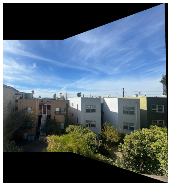
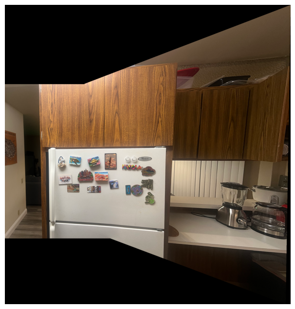
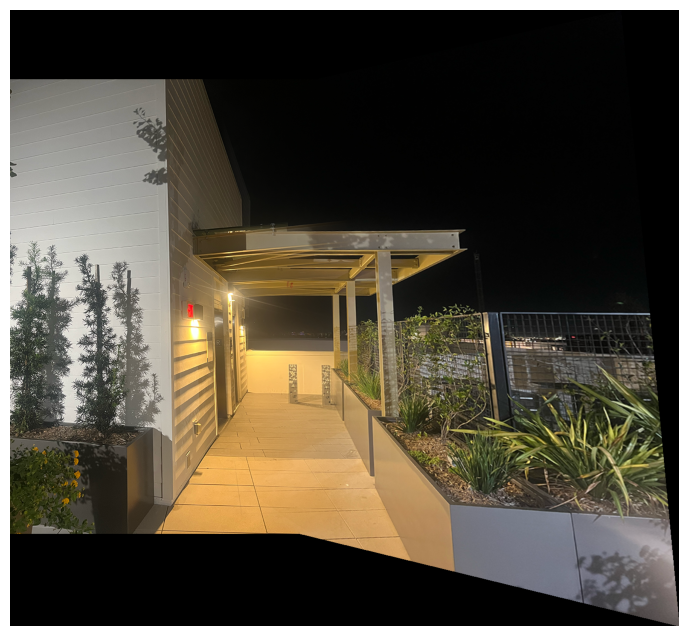
After computing homographies with RANSAC, I ran the same code that I used for part A to produce mosaics for the same 3 pictures. Here are the side-by-side manually and automatically stitched results for these images:

Manual Stitching

Automatic Stitching

Manual Stitching

Automatic Stitching

Manual Stitching

Automatic Stitching

I think with automatic stitching, the results were better. I may have done a few slightly inaccurate point correspondences, and this may have affected manual stitching results. The coolest thing I learned while doing the project was implementing the RANSAC algorithm from scratch. Even though I took introduction to machine learning class before, I haven't had the chance to code RANSAC and I think it was cool to learn how to code its iterative consensus algorithm.