Project 5: Fun With Diffusion Models!

Alp Eren Ozdarendeli

Part 0: Setup

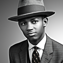
For the setup part, I use DeepFloyd IF as the diffusion model. For Part A, I used the seed 180. Deepfloyd is a two-stage model. In the first stage, 64 x 64 images are produced and second stage takes these images and produces final images of size 256 x 256. To test the setup, I used the given prompts to generate the following outputs:

a man wearing a hat

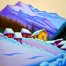
an oil painting of a snowy mountain village

a rocket ship

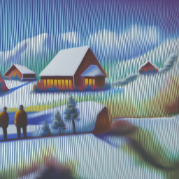
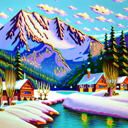
The generated images actually represent the prompts pretty well. To test the effect of num_inference_steps on the outputs, I test the prompt 'an oil painting of a snowy mountain village' with num_inference_steps 7 and 46 in addition to 20 given above. Here are outputs with num_inference_steps 7 and 46 respectively:

an oil painting of a snowy mountain village (num_inference_steps = 7)

an oil painting of a snowy mountain village (num_inference_steps = 46)

With increasing num_inference_steps, the images become more detailed and better reflect the prompts.

1.1 Implementing the Forward Process

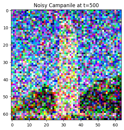
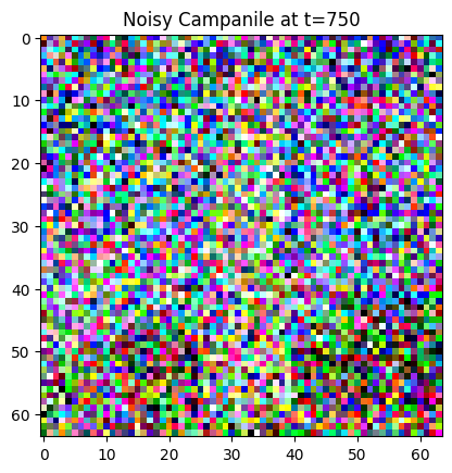
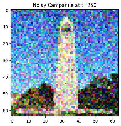
Now, I implement the forward process. For the forward process, given a clean image, I get a noisy image for a timestep t by sampling noise from a Gaussian. In addition to these, I also scale the image. The original Campanile image is shown below at different noise levels. Larger t represents larger noise.

Noisy Campanile at t=250

Noisy Campanile at t=500

Noisy Campanile at t=750

1.2 Classical Denoising

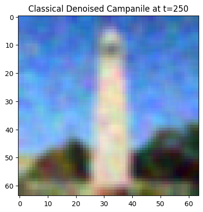
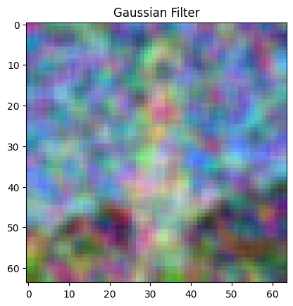
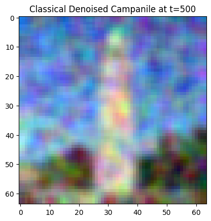
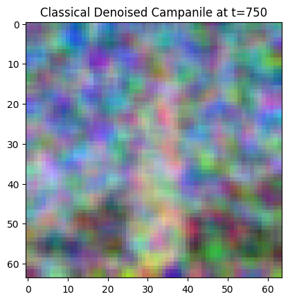
In this section, I use classical denoising to denoise the noisy images produced in the previous part. For classical denoising, I take a noisy image and try to denoise it by Gaussian filtering. Here are the results for different timestamps:

Noisy Campanile at t=250

Noisy Campanile at t=500

Noisy Campanile at t=750

Classical Denoised Campanile at t=250

Classical Denoised Campanile at t=500

Classical Denoised Campanile at t=750

1.3 One-Step Denoising

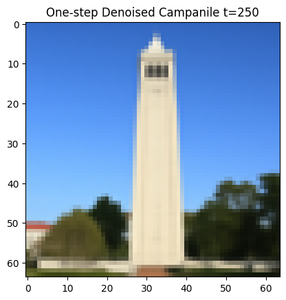
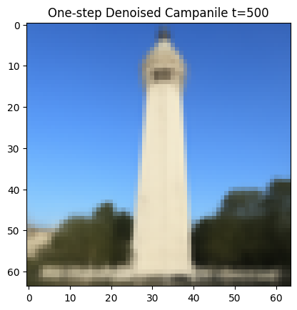
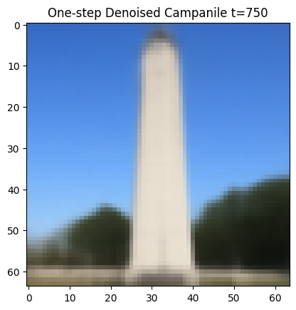
For one-step denoising, I use a pretrained denoiser stage_1.unet to find the noise in the images. This UNet is already trained on a very large dataset but it was trained text conditioning so I use the embedding of the given prompt "a high quality photo” for conditioning. Then, I remove this image to recover a clean image for noisy images produced in part 1.1:

Noisy Campanile at t=250

Noisy Campanile at t=500

Noisy Campanile at t=750

One-Step Denoised Campanile at t=250

One-Step Denoised Campanile at t=500

One-Step Denoised Campanile at t=750

1. 4 Iterative Denoising

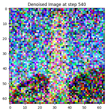
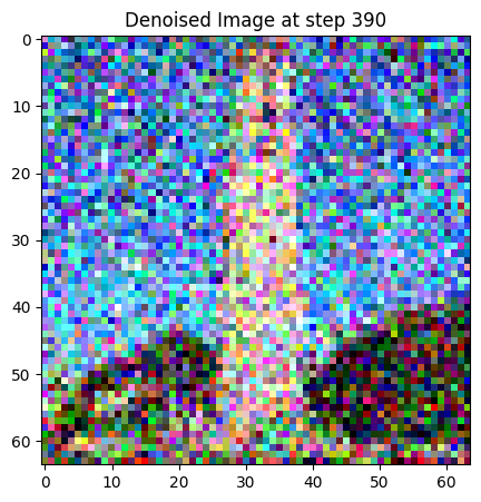
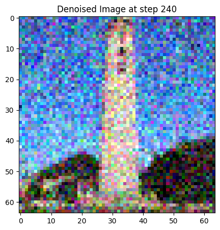
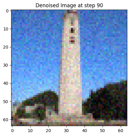
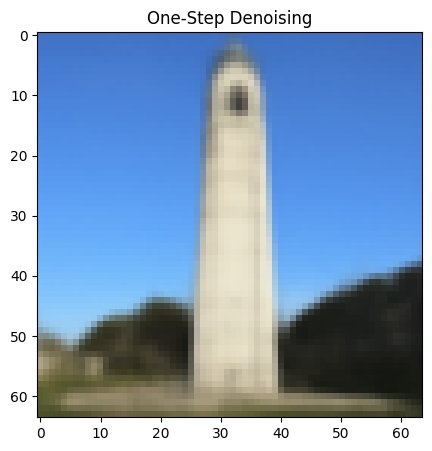
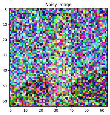
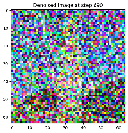
In the previous part, performance gets worse with more noisy images. To combat this, I will implement iterative denoising. For iterative denoising, I create a new list of timesteps,strided_timesteps, to skip some steps. The stride of steps will be 30. I add noise to the test image at timestep[10] and run the implemented iterative_denoise function on this image with i_start algorithm being 10. In the following, denoised image is displayed at every fifth step and final clean image prediction is shown in comparison to other techniques:

1.5 Diffusion Model Sampling

For this part, I use iterative_denoise function I defined earlier to generate images from scratch by passing 0 as the i_start argument. I also pass in random noise, and the function denoises pure noise. Here are 5 samples with the prompt “a high quality photo”:

1.6 Classifier-Free Guidance (CFG)

The quality of the results in the previous section were not great. To significantly improve image quality, I will use CFG in this section. For CFG, I compute both conditional and unconditional noise estimate. In CFG, we have a hyperparameter, named scale in the function, that determines its strength. When scale is 0, CFG is essentially unconditional noise estimate but when scale is bigger than 1, CFG can produce much more quality images. Here are 5 samples from CFG with scale=7 and prompt “a high quality photo”:

1.7 Image-to-image Translation

In this section, I follow the SDEdit algorithm. I noise the original image a little bit first, then, force it back to the image manifold without conditioning. As a result, I get an image similar to the original image. For this section, I will use the 3 test images, one of them being the Campanile photo. Here are the edits of the test images, at different noise levels 1, 3, 5, 7, 10, 20 with "a high quality photo":

i_start=1

i_start=3

i_start=5

i_start=7

i_start=10

i_start=20

Original Campanile

i_start=1

i_start=3

i_start=5

i_start=7

i_start=10

i_start=20

Original Golden Gate

i_start=1

i_start=3

i_start=5

i_start=7

i_start=10

i_start=20

Original cat

1.7.1 Editing Hand-Drawn and Web Images

The technique I used in the previous section also performs pretty well for nonrealistic images that is projected it to the natural image manifold. To test for these, I will use 1 image from web and 2 images by my hand drawing:

i_start=1

i_start=3

i_start=5

i_start=7

i_start=10

i_start=20

Original UP

i_start=1

i_start=3

i_start=5

i_start=7

i_start=10

i_start=20

Original Hand Drawing 1

i_start=1

i_start=3

i_start=5

i_start=7

i_start=10

i_start=20

Original Hand Drawing 2

1.7.2 Inpainting

Based on the Repaint paper, I implement inpainting in this section using the same procedure. Given a mask, when I run the diffusion denoising loop, I replace everything except the mask area with the original images but with the added noise based on timestep t. So, new content is only produced in the pixels where mask has value 1. Here are my results for inpainting:

Original

Mask

To Replace

Final

Original

Mask

To Replace

Final

Original

Mask

To Replace

Final

1.7.3 Text-Conditional Image-to-image Translation

In this section, I will do text conditional image to image translation. It is pretty much the same with SDEdit. Differently from the original SDEdit, I will change the prompt from "a high quality photo" to the prompt of my choosing to guide the projection with text prompt. Here are the results with different noise levels and different prompts:

i_start=1

i_start=3

i_start=5

i_start=7

i_start=10

i_start=20

Original Campanile

i_start=1

i_start=3

i_start=5

i_start=7

i_start=10

i_start=20

Original Cat

i_start=1

i_start=3

i_start=5

i_start=7

i_start=10

i_start=20

Original Red-Eyed Frog

1.8 Visual Anagrams

In this section, I will implement visual diagrams. Visual anagrams are images such that the image looks like a prompt —prompt1— upright, but looks like another prompt —prompt2— when it is turned upside down. I implement visual anagrams by denoising the image at a timestep t with prompt1 and get a noise estimate e_1. Then, I turned the image upside down, denoise the flipped image with prompt2 to get a noise estimate e_2. Finally, I turned e_2 upside down and took its average with e_1 with to get the final noise estimate. The denoising step is done with this final noise estimate. Here are my results, and prompts:

"an oil painting of people around a campfire"

"an oil painting of an old man"

"an oil painting of an octopus in the wavy sea"

"an oil painting of a curly hair man"

"a painting of a santa claus"

"a painting of a deer"

1.9 Hybrid Images

In this section, I will implement hybrid images implementation. Hybrids images appear as a prompt from afar, and as another prompt from a closer range. To create hybrid images, I will use a similar technique to the previous section. I will first estimate the noise with two different prompts, and will pass them through low-pass filter. Then, I will combine the low frequency component of one noise with the high frequency component of the other noise. Their combination will form the final noise estimate. Here are my results by using Gaussian blur with kernel size 33 and sigma 2:

'a lithograph of a skull' and 'a lithograph of waterfalls'

"a lithography of frog" and "a lithography of autumn leaves"

"a lithography of Batman symbol" and "a lithography of a city with skyscrapers"

Part B: Diffusion Models from Scratch

Training a Single-Step Denoising UNet

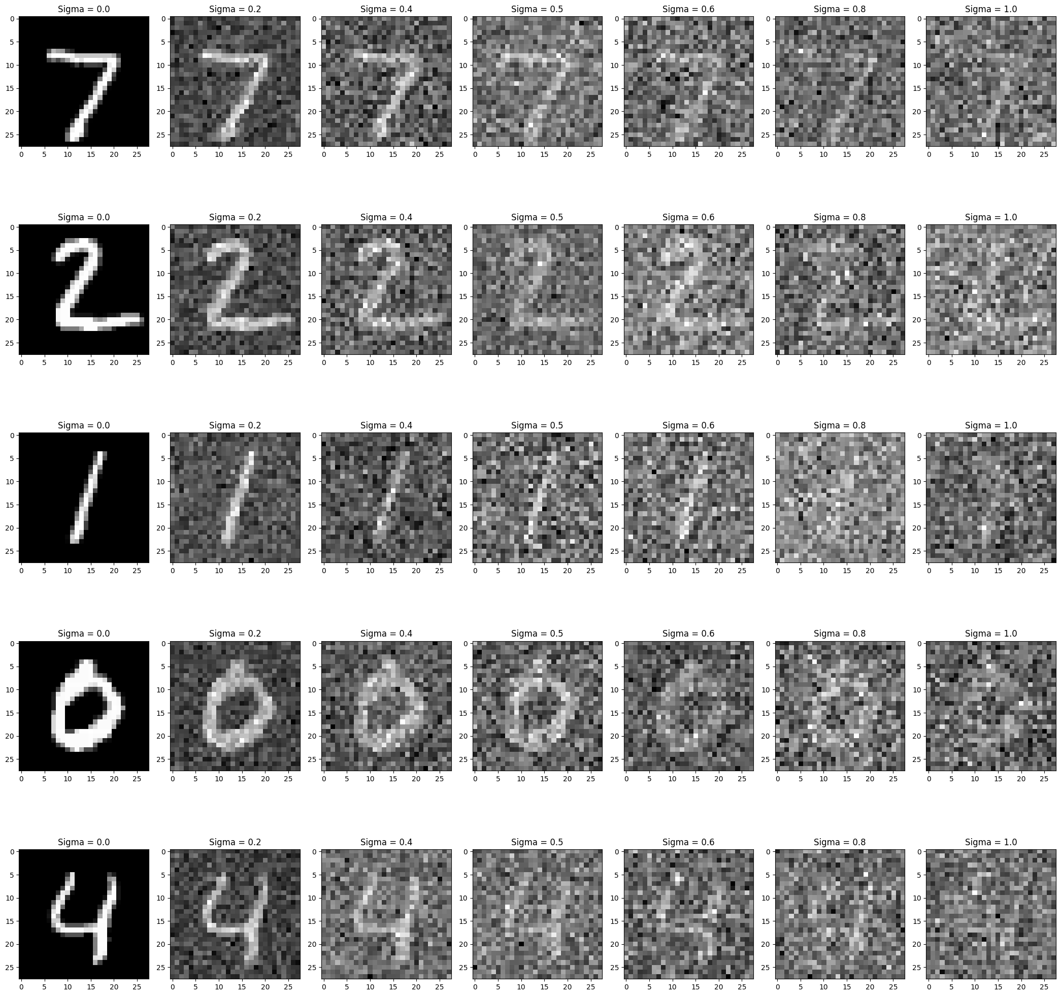
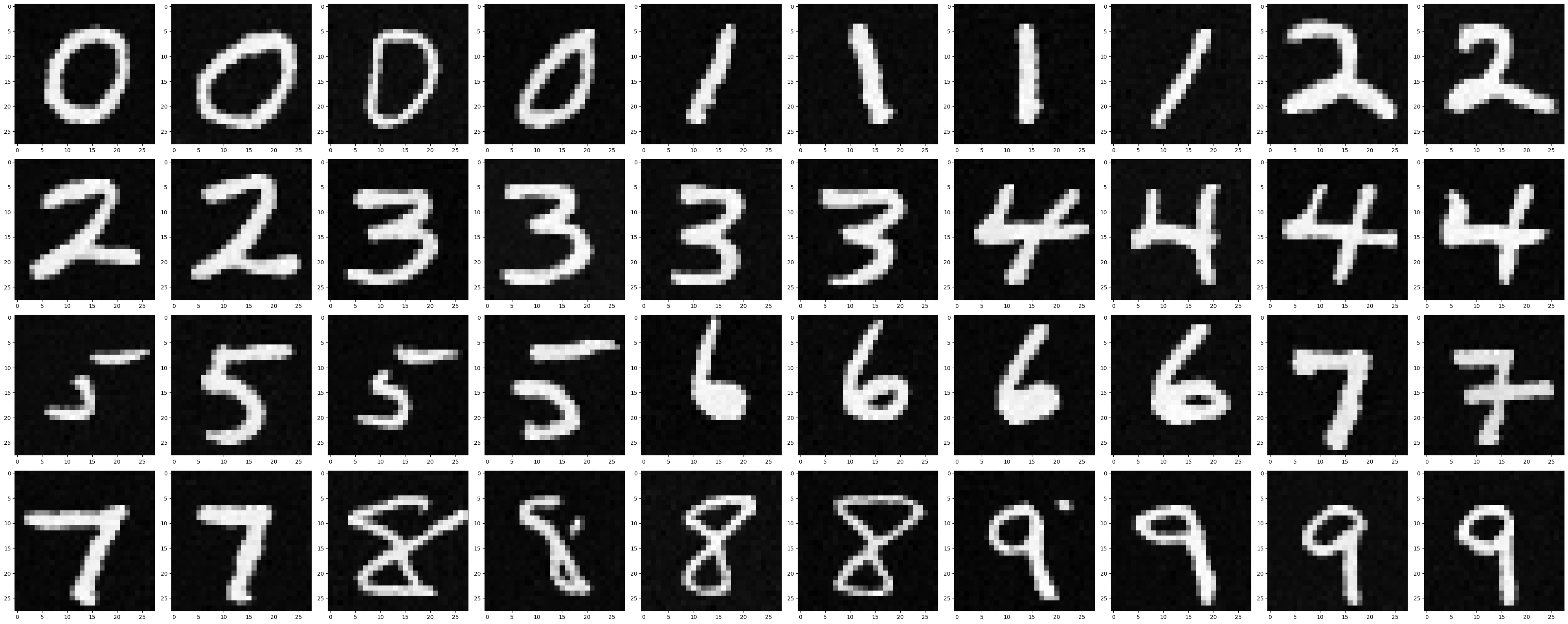
For the second part of the project, I implement diffusion models from scratch. As a first step, I train single-step denoising UNet. This denoiser will optimize for producing a clean image given a noisy image. Firstly, I follow the model diagram for UNet to define its architecture. To train a denoiser with UNet, I use the image dataset from MNIST. Given a clean image, I add a random noise with sigma coefficient to create a noised image. Here are examples of noised images with different sigmas:

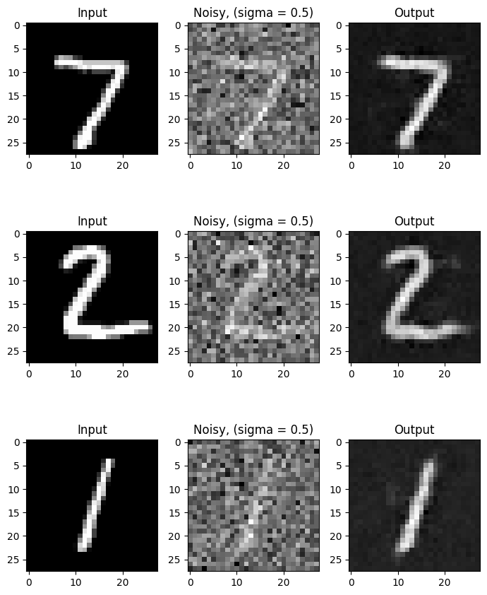
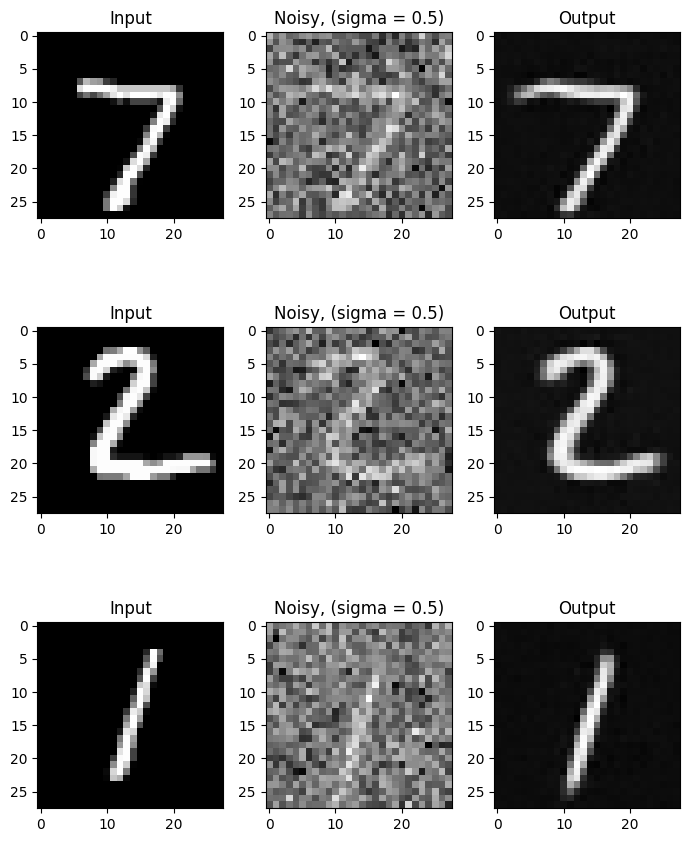
I train UNet to minimize the loss between denoised image from UNet given the noised image and the original clean image. I shuffle the training dataset before creating its data loader. In this part, I will be using hidden dimension of 128 and learning rate of 1e-4 for Adam optimizer. Here are the sample results after training for 1 and 5 epochs:

In the training, I train the model for sigma = 0.5. Here is how the model performs for other sigma values that it wasn’t exactly trained for:

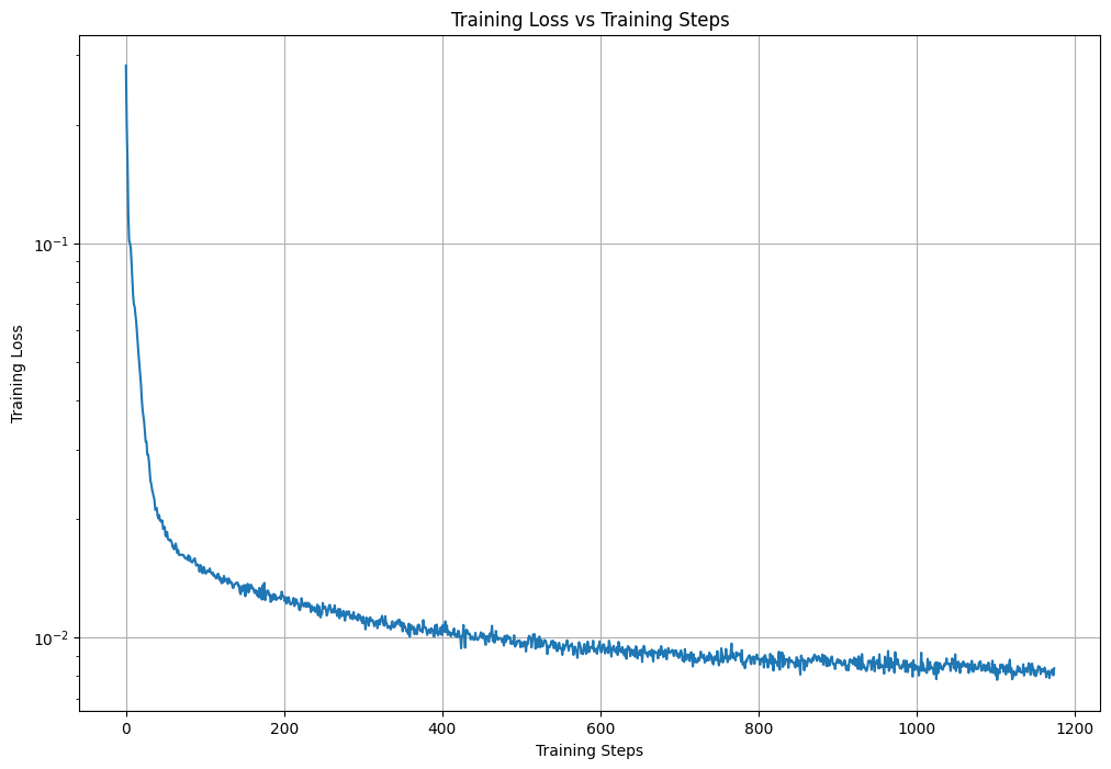
Here is the training loss curve during the whole training process:

Training a Diffusion Model

In this part, I will train a UNet model that iteratively denoises an image. For this, I will implement DDPM. For this part, our optimization problem is not the same as the previous part., even though they are mathematically equivalent In this part, I UNet predicts the added noise rather than the clean image itself. In order to get a quality result, we need to iteratively denoise the image. Thus, following the diagram and using FCBlocks, I inject time t into the UNet model architecture for conditioning. To train the model, I pick a random image from the training set data loader, pick a random t, and train the denoiser for computing the noise of the image at timestep t. In This section, I use hidden dimension of 64, initial learning rate of 1e-3 for Adam optimizer, and gamma of 0.1 ** (1.0/num_epochs) for exponential learning rate decay scheduler.

Also, during training I sample the model for 5 and 20 epochs:

2.4 Adding Class-Conditioning to UNet

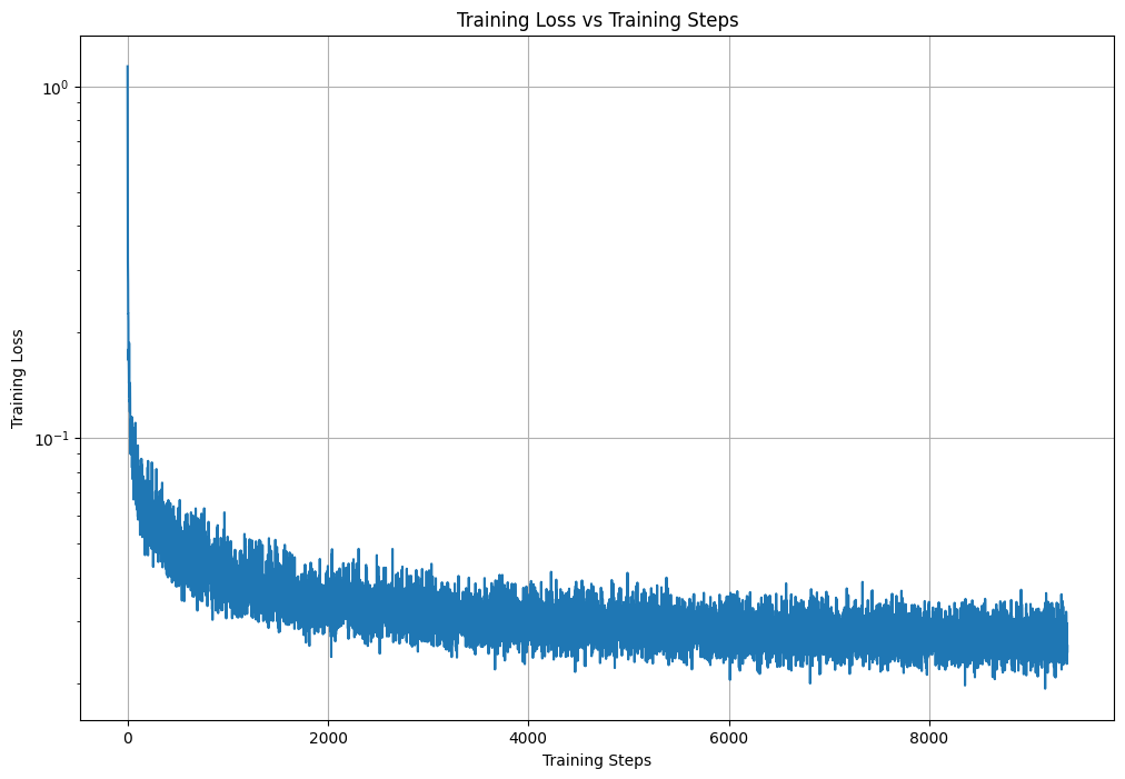
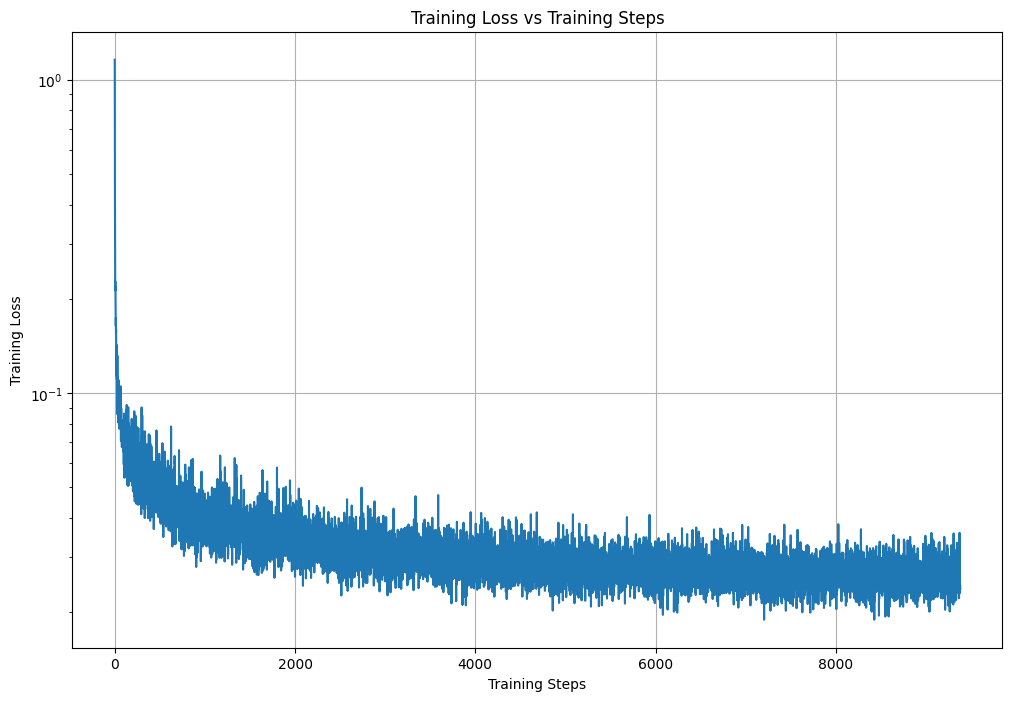
In order to improve our results from the previous section, I will add class-conditioning to UNet in this section by adding 2 more FCBlocks to the UNet architecture. Class-conditioning vector— one-hot vector c— will be set to 0 %10 of the time by implementing p_uncond = 0. 1. Training hyper parameters are basically the same as the previous section. Here is the training curve for the training process:

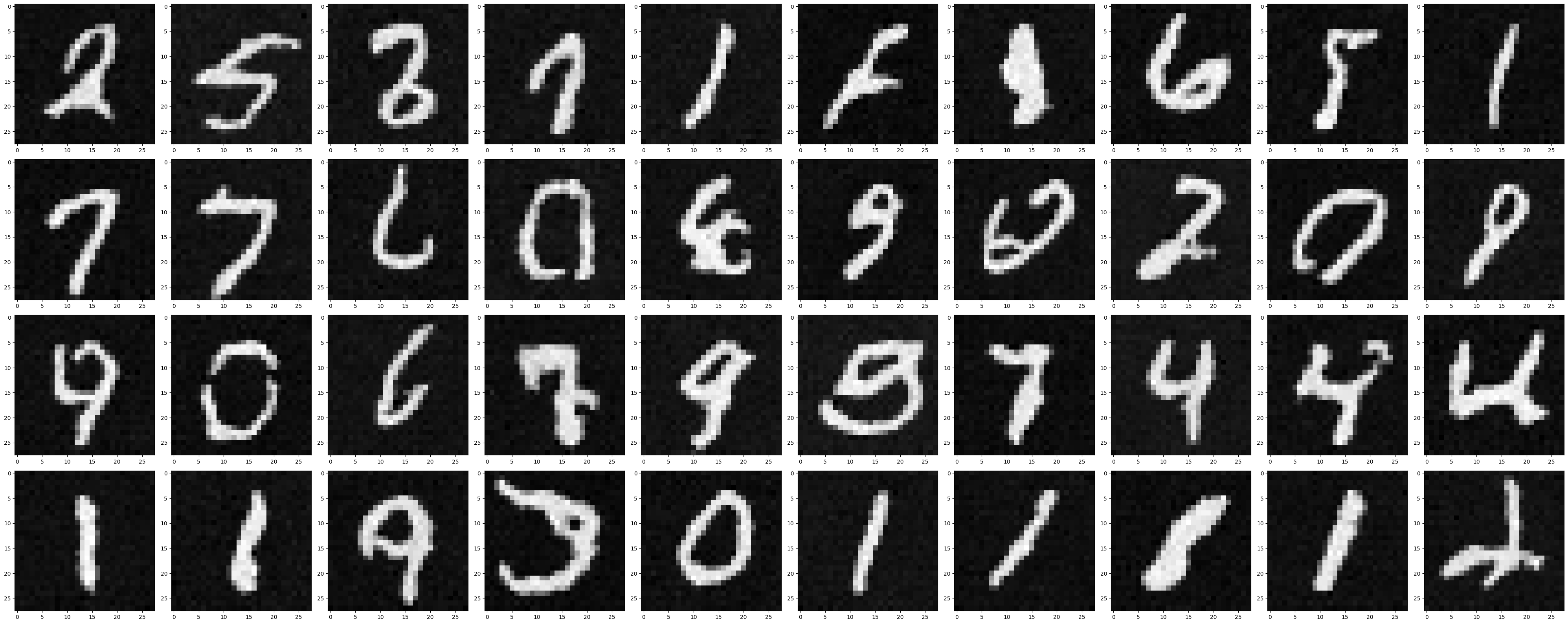
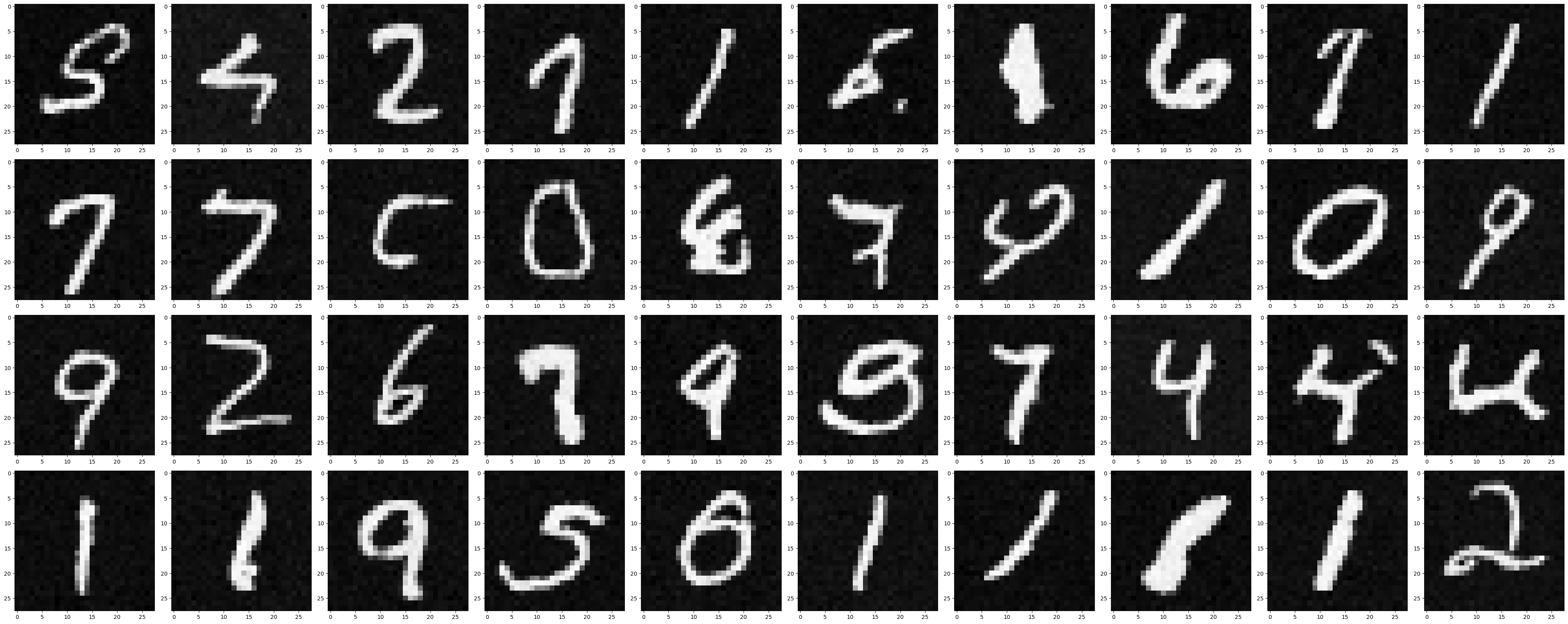
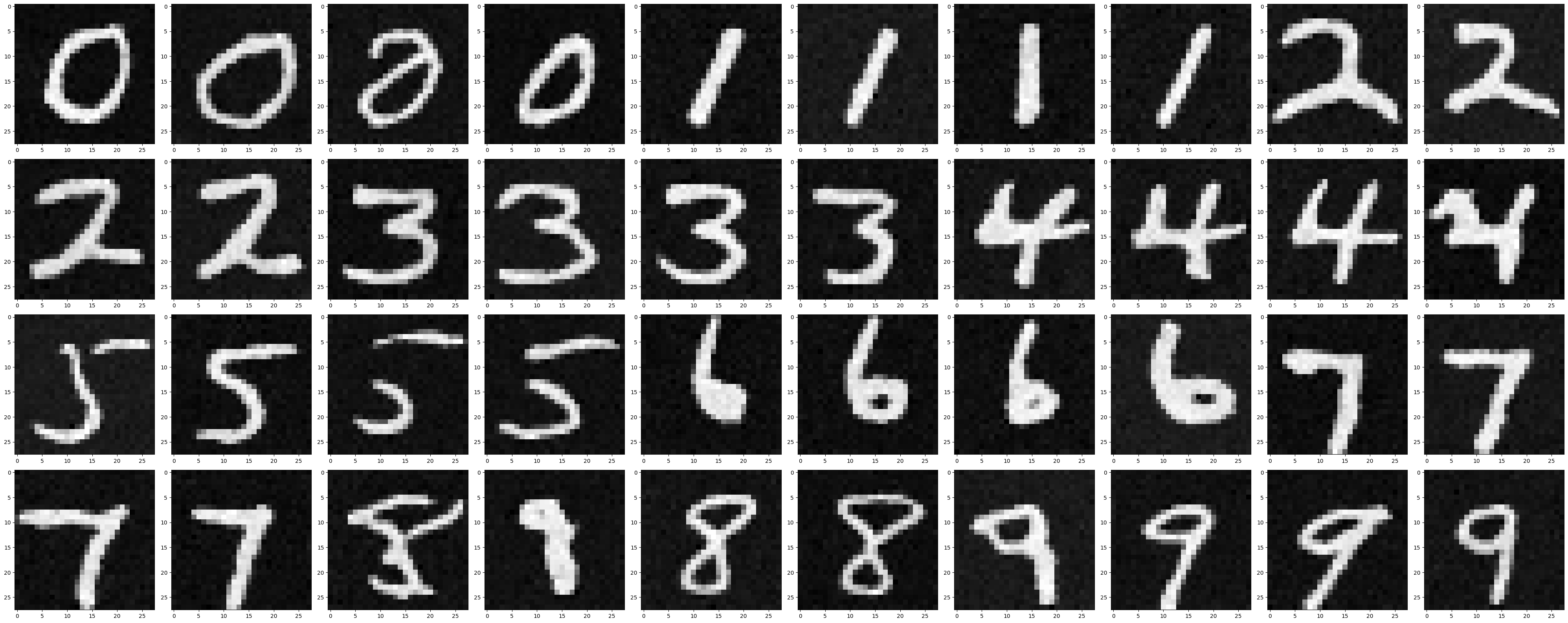
Now, I sample the class-conditioned UNet for 5 and 20 epochs Here is the result for 4 instances of each digit at 5 and 20 epochs: